v2206: New and improved pre-processing
TOP
snappyHexMesh has been extended to optionally perform automatic hole closure if unreachable locations (locationsOutsideMesh) have been specified. In previous snappyHexMesh versions, a leak-path for visualisation was written and the meshing process aborted with an error message if any connections between inside points and outside points were identified.
The hole closure algorithm is based on "A 3D-Hole Closing Algorithm" by Zouina Aktouf et al, which determines the convex hull (in terms of mesh faces) needed to close a gap. Any point on these added faces is added to the pointZone frozenPoints and is excluded from any snap-to-nearest-surface, and smoothed only. Note that there is no special handling for layer addition on the added faces.
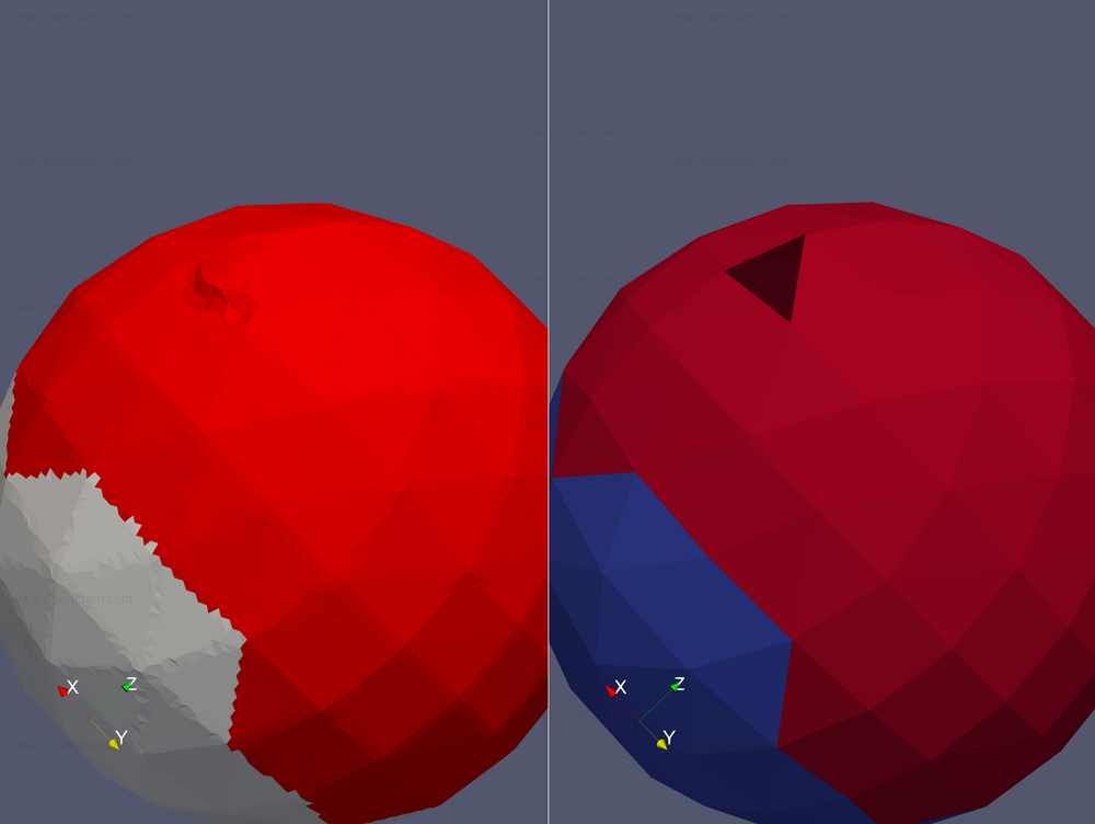
An example is given below, where the original geometry (on the right) has a missing triangle. The gap is subsequently closed and smoothed in the snapping phase (figure on the left). In this example the gap is closed with faces across different refinement levels (since the mesh was refined only at the surface) and hence the smoothing is not perfect.
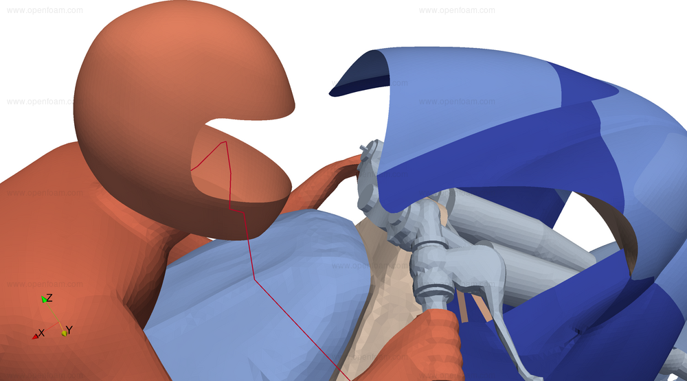
A more extreme example is shown below, based on the motorBike tutorial where the visor of the helmet has been removed. The surface with the leak path is shown in red:
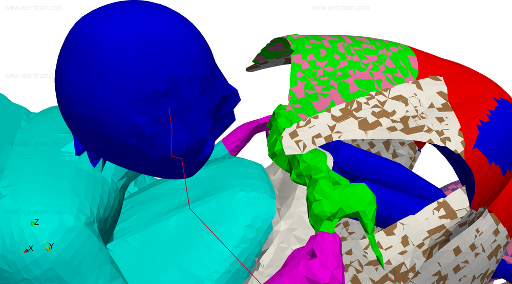
After leak closure, the following mesh is generated:
As can be seen the resulting mesh is far from smooth - the algorithm should only be used to close small gaps.
Usage
The new functionality is enabled in the castellatedMeshControls section of the snappyHexMeshDict by adding the entry:
useLeakClosure true;
- any leak paths identified are written to a leakPath Ensight file in the postProcessing directory
- an optional user input, leakLevel, specifies on a per-surface, per-region basis at what cell level the leak detection kicks in. This permits 'early' closure of leak paths to limit the maximum number of cells during the intermediate refinement levels, but at the cost of using coarse faces to block the gap. This may also report false positives if the mesh is still so coarse that the inside and outside locations are still in the same cell.
refinementSurfaces
{
    "sphere.*"
    {
        // Surface-wise min and max refinement level
        level (6 6);

        // Optional level at which to start early checking for leaks
        leakLevel 2;
    }
    ...
See also
- holeToFace faceSet source. This allows use of the algorithm on any existing mesh using topoSet. See $FOAM_ETC/caseDicts/annotated/topoSetSourcesDict.
Tutorials
- $FOAM_TUTORIALS/mesh/snappyHexMesh/sphere_gapClosure (missing triangle in triangulated sphere)
- $FOAM_TUTORIALS/mesh/snappyHexMesh/motorBike_leakDetection (missing section of input surface)
Source code
TOP
blockLevel memory usage
In version v1912 automatic closure of thin gaps was introduced through the optional entry blockLevel:
refinementSurfaces
{
    "gap.*"
    {
        // Surface-wise min and max refinement level
        level       (2 2);

        // From cell level 2 onwards start checking
        // for opposite surfaces
        blockLevel  2;
    }
}
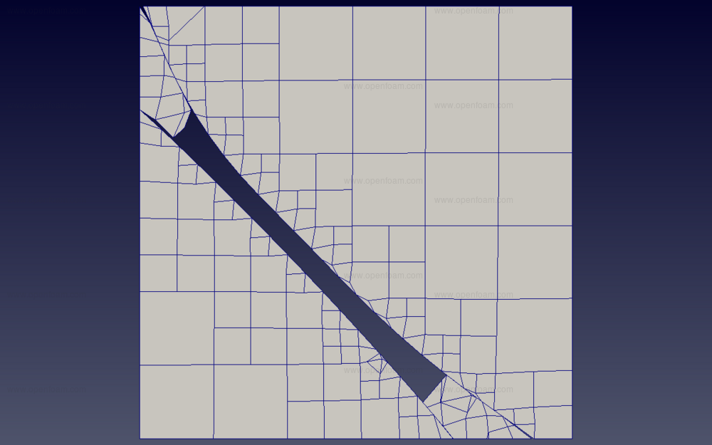
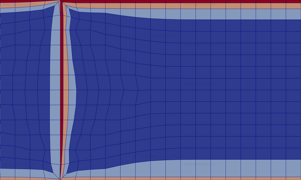
For example, in the opposite_walls tutorial, cells in the thin gap between the two surfaces are identified and removed:
In previous versions this was performed in two passes:
- determine wall distance by walking through the mesh starting from each surface
- for all cells, for each combination of surfaces, determine if the cell is inside the gap
This split has severe memory and performance limitations when operating on large surfaces and large meshes since all the information from pass 1 needs to be stored. In the new implementation the wall distance walking stops if it has walked more than the allowed maximum gap size, leading to dramatically less data transfer.
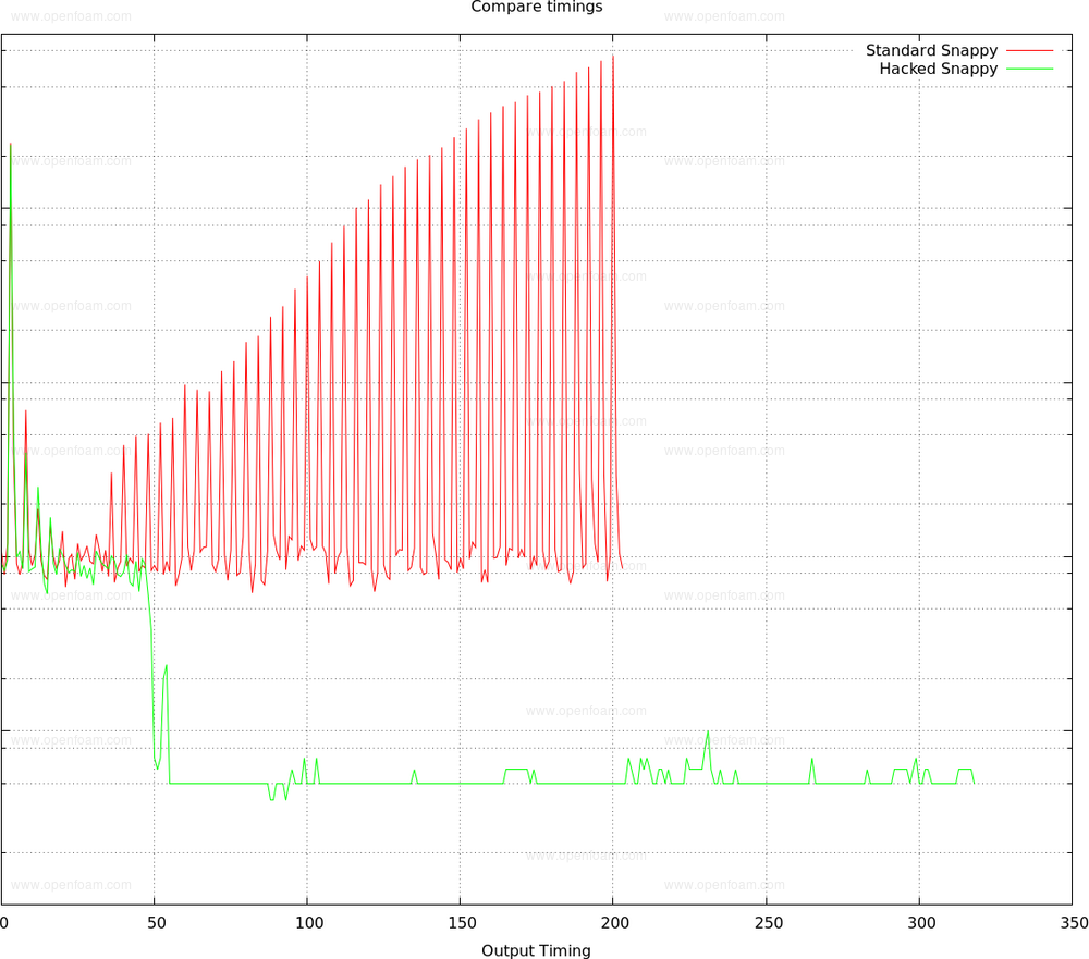
The figure below compares the amount of memory (y-axis) v.s. iteration (x-axis) for v2112 ('Standard Snappy') memory usage to the new implementation ('Hacked Snappy'). Memory usage for the old implementation keeps on increasing until the memory is exhausted; the new implementation successfully removes the unreachable cells (around step 50) and returns the memory to the system.
Parallel consistent faceZones
Parallel behaviour was stress-tested by comparing 'standard' runs against the random decomposition method. This highlighted slight differences in the faceZone allocation algorithm due to not handling faceZones that coincide with processor patches. There may still be areas which are not exactly the same due to e.g. truncation errors in calculating the face- and cell-centres due to different point ordering or orientation of face on processor patch, different ordering of faces in cell etc.
Tutorials
Source code
TOP

Instead of adding layers in a single pass, snappyHexMesh can now use multiple passes. This gives more opportunity to the mesh shrinking phase to make space for extra layer(s). The new behaviour is enabled with the new nOuterIter keyword in the layerParameters section of the snappyHexMeshDict:
// Outer loop iterations (each of which is up to nLayerIter). Default is 1.
nOuterIter      3;
This setting divides the total number of layers across these iterations, e.g. if 20 layers are requested, these will be added in 3 passes with 7, 7 and 6 layers per pass.
- the nOuterIter entry can be set to a large number to cause the layers to be added one-by-one.
- the outer loop will exit if no cells-to-be-added are left or if none can be added, e.g. due to quality constraints.
-
it is generally recommended to switch off the gradual layer termination to avoid every outer iteration causing additional growth where no layers are added:
nGrow -1; - the expansionRatio and minThickness are calculated once and then kept constant across the outer iterations.
-
when outputting the layer coverage fields:
writeFlags
(
    layerFields     // write volScalarField for layer coverage
);
The resultant field shows the sum of cells added per added cell. An example is given below, taken from the mesh/snappyHexMesh/addLayersToFaceZone tutorial, where each of the three passes adds a single layer. Here, cells added in pass 1 have value 1, those added in pass 2 have value 2 etc.
Effect on layer addition
The effect of employing multiple passes on the layer addition process is highlighted below, using a sphere geometry with two regions, resulting in two patches (sphere_patch0, sphere_patch1). Running without nOuterIter, i.e. adding all layers in one go yields:
With nOuterIter 3, i.e. adding layers one by one:
The effect of using multiple passes for this case is a slightly better coverage:
| nOuterIter | patch | nLayers |
|---|---|---|
| 1 | sphere_patch0 | 2.38 |
| sphere_patch1 | 2.7 | |
| 3 | sphere_patch0 | 2.62 |
| sphere_patch1 | 2.91 |
Tutorials
Source code
TOP
The holeToFace face source, usable in e.g. topoSet, generates the minimum set of faces to close the gap between two mesh regions. It uses the algorithm as described in "A 3D-Hole Closing Algorithm", by Zouina Aktouf et al. A typical use in a topoSet dictionary might be
source  holeToFace;
points
(
    ((0.2 0.2 -10) (1.3 0.4 -0.1))  // points for zone 0
    ((10 10 10))                    // points for zone 1
);
The algorithm
- marks all boundary faces and any faces in an optional faceSet
- determines if there are any connections between the zones (indicated by the specified points)
- determines the minimum set of internal/coupled faces that closes the hole/disconnects the zones
The underlying algorithm is used in the new automatic hole closure in snappyHexMesh.
Tutorials
- $FOAM_TUTORIALS/mesh/snappyHexMesh/gap_detection (gap detection)
Source code
TOP
createPatch has been extended to include handling of fields, and automatic re-patching of matching faces, both between different regions and on a single region.
Handling of fields
Users can now specify boundary conditions for the newly added patches, similar to createBaffles. This is generally not required for constraint-type patches, e.g. cyclic, since these automatically use the relevant constraint boundary condition. The boundary condition addition is activated by the presence of the patchFields subdictionary:
// Dictionary to construct new patch from
patchInfo
{
    type        patch;

    //- Optional override of added patchfields. If not specified
    //  any added patchfields are of type calculated.
    patchFields
    {
        T
        {
            type            uniformFixedValue;
            uniformValue    300;
        }
    }
}
Note that the patch fields are created when the patches still have zero faces, meaning that any patch field not fully specified by the dictionary will not be initialised correctly, e.g. mixed and hence turbulentTemperatureRadCoupledMixed.
Automatic patching
The selection of faces to re-patch has been extended to include automatic overlap calculation:
// How to select the faces:
//  - set : specify faceSet in 'set'
//  - patches : specify names in 'patches'
//  - autoPatch : attempts automatic patching of the specified
//                candidates in 'patches'.
//      - single region : match in the region itself
//      - multi regions : match in between regions only
constructFrom autoPatch;
With autoPatch:
- regions are provided as command line options, e.g. autoPatch -allRegions (reads the constant/regionProperties file)
- each region has to provide its own system/<region>/createPatchDict, though quite often these can be links to the same file.
- when applied to multiple regions, automatic patching is restricted to patch coupling across different regions.
- a single set of faces can now become multiple patches so the name entry is used as a prefix. The actual patch name becomes <name><region1>_to_<region2>.
- the name entry can be left out to remove the prefix (dictionaries do not support empty words)
- the automatic matching of faces employs the AMI framework. It uses the faceAreaWeightAMI method (this can be overwritten in the patchInfo dictionary) to detect faces which are overlapping other patches more than 50% and automatically generates a patch for these and moves the faces across. It also moves across any donor faces on the corresponding region. This can give problems if a face is donor to multiple patches where the first AMI 'wins'.
- the faceAreaWeightAMI and faceAreaWeightAMI2D methods have been extended to allow specification of a maximum match distance (and face-normal alignment). The default method is extremely relaxed about which faces match so these settings might be necessary where there are close differing matches. Note that none of the existing AMIMethods handle obscured patches.
- to check weights of faceAreaWeightAMI and faceAreaWeightAMI2D the checkMesh utility has been extended so the -allGeometry option also outputs weights on the mapped boundaries, e.g. the following command will write the weights to the postProcessing directory.
checkMesh -allRegions -allGeometry
- the source patches can also be provided as patch groups. This can be convenient for multi-region cases, whereby the same createPatchDict can be applied to all regions.
- the automatic patching can make it a lot easier to set up CHT cases. The mappedPatch or mappedWall type patches can both use AMI and so have consistent behaviour to the face repatching:
// Dictionary to construct new patch from
patchInfo
{
    type        mappedPatch;
    sampleMode  nearestPatchFaceAMI;
    AMIMethod   faceAreaWeightAMI2D;

    patchFields
    {
        T
        {
            type            compressible::turbulentTemperatureRadCoupledMixed;
            Tnbr            T;
            kappaMethod     solidThermo;
            value           uniform 300;
        }
    }
}
Please note that the patchField specification above will actually not work correctly because of the aforementioned zero-faces on the patch.
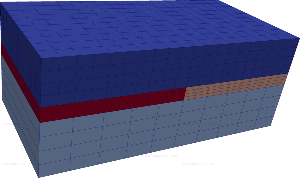
A simple tutorial has been assembled with a single solid region at the bottom (light blue), two smaller solid regions (red, orange) in the middle and a fluid region at the top (blue):
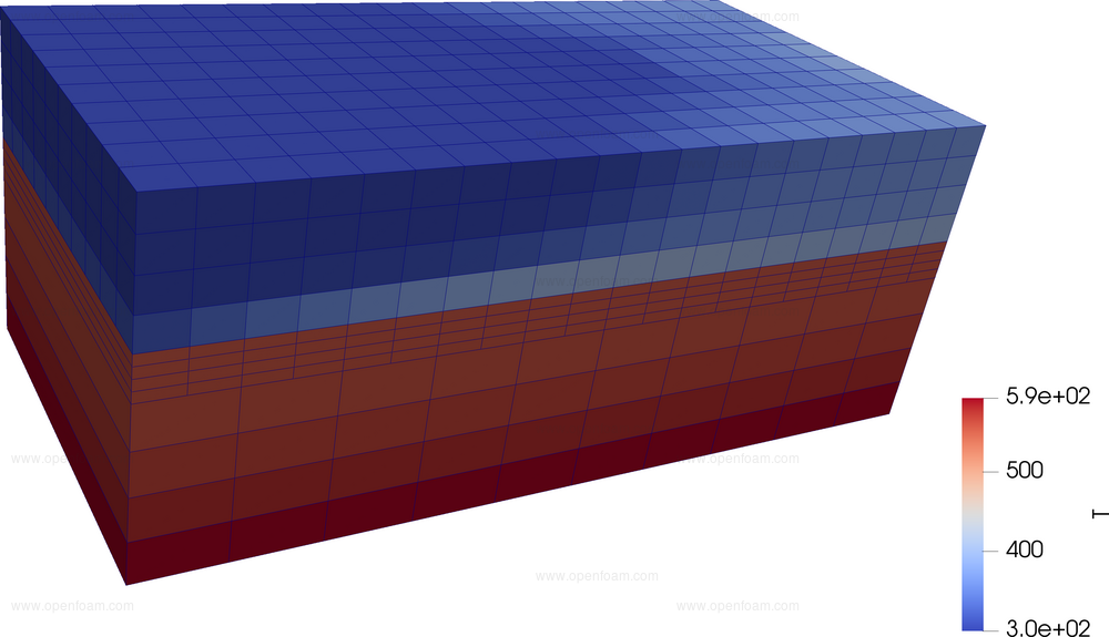
Temperature distribution (bottom of the bottom region is heated, top region has flow from left to right)
Tutorials
- $FOAM_TUTORIALS/mesh/createPatch/multiRegionHeater_autoPatch (automatic patching of a CHT case)
Source code
- $FOAM_UTILITIES/mesh/manipulation/createPatch
- $FOAM_UTILITIES/mesh/manipulation/checkMesh (writing mapped weights)
TOP
When using a triSurfaceMesh in e.g. topoSet with searchableSurfaceToFace, the code would identify whether the surface is closed by checking if all edges are used by two faces, e.g. in topoSetDict
actions
(
    {
        name            collectorSet;
        type            faceSet;
        action          new;
        source          searchableSurfaceToFace;
        surfaceType     triSurfaceMesh;
        surfaceName     mySurface.obj;
    }
);
An additional check has been added to see if the two faces have consistent orientation. If the check fails, a warning message will be issued:
--> FOAM Warning :
    From bool Foam::triSurfaceMesh::isSurfaceClosed() const
    in file searchableSurfaces/triSurfaceMesh/triSurfaceMesh.C at line 255
    Surface mySurface.obj is closed but has inconsistent face orientation
    at edge (0.97205 -0.46948 0.64841)(0.97167 -0.4683 0.64911)
    This means it probably cannot be used for inside/outside queries. Suppressing further messages.
Note that a similar check is also in the surfaceCheck application:
Number of zones (connected area with consistent normal) : 2
More than one normal orientation.
This topological error can be corrected using the surfaceOrient application.
Source code
TOP
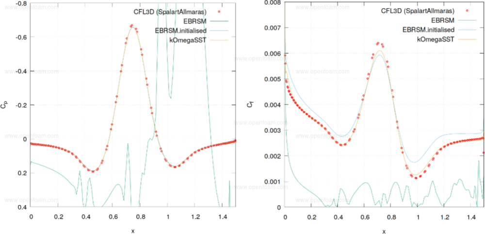
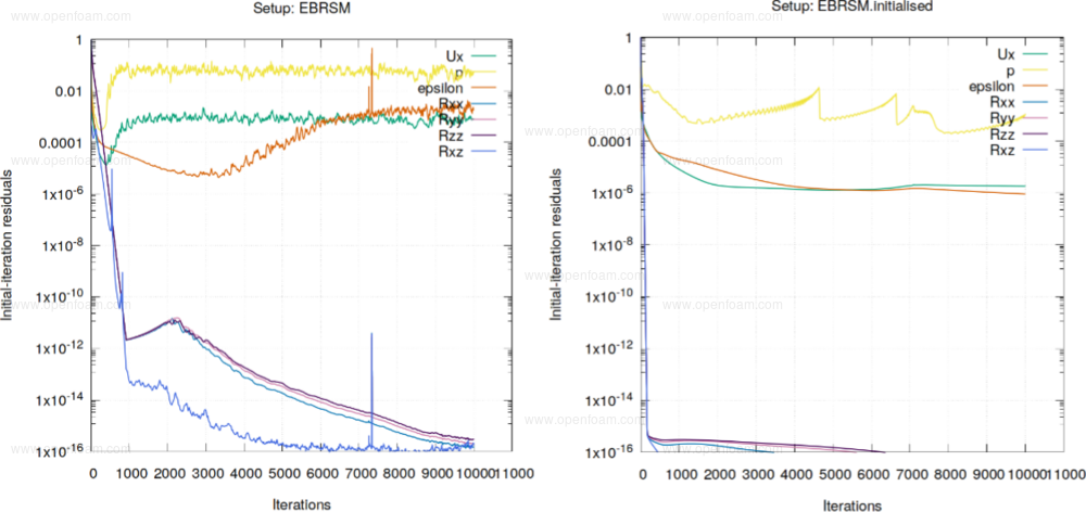
As Lardeau and Manceau (2014) noted:
One of main issues faced when using many RANS models is the slow or non-convergence in the initial stage of the computation. This is particularly restrictive for low-Re model, and it has been attributed to a bifurcation property inherited from the low-Reynolds damping formulation. Rumsey et al. (2006) showed that alternative converged solutions could be obtained, depending on the initial and inflow conditions.
To address this issue, a new preprocessing utility called setTurbulenceFields has been implemented based on Manceau's two-step automatic initialisation procedure for RANS computations.
setTurbulenceFields only requires the reference speed of the flow as an input. It can optionally initialise turbulence fields, e.g. epsilon, and/or a velocity field, and can help to improve convergence in the first O(10) time steps and the fidelity of results.
The positive effects of initialisation by setTurbulenceFields can be seen in the NASA's 2D Bump-in-channel case when employing the new elliptic-blending Reynolds stress turbulence:
Source code
Tutorial
Merge request
References
- Manceau, R. (n.d.). A two-step automatic initialization procedure for RANS computations. (Unpublished).
Attribution
- OpenCFD would like to acknowledge and thank Prof. Rémi Manceau for providing the governing equations for setTurbulenceFields, elaborate suggestions and critical recommendations.