The radiation view factor generation application, viewFactorsGen, has received multiple updates:
The method is now based on a combination of double area integral (2AI) when the two surfaces are 'far' apart, and double linear integral (2LI) when surfaces are 'close'. The distance between faces is calculated as the ratio between average areas and the distance between face centres;
Default use of the standard iterative linear solvers in OpenFOAM, versus the earlier direct solution on a single processor; and
If compiled with CGAL support, a faster ray intersection routine can be applied.
Dictionary inputs
Additional inputs in the viewFactorsDict dictionary comprise:
// GaussQuad integral error tolerance (default: 0.01)
// Used to decide when to increase order of integration.
GaussQuadTol              0.1;

// Relative distance (default: 8)
// For distTol : use 2AI
distTol                   8;

// Constant model use for common edges for 2LI (default : 0.22)
// Approx for integral value of duplicate edges.
alpha                     0.22;

// Interval tolerance (default : 1e-2)
// Used for ray shooting from face centre to face centre plus intTol to avoid the ray
// hitting the same face where it was originated.
intTol                    1e-2;
The use of iterative versus direct linear solver is specified using the optional useDirectSolver entry in the radiationProperties dictionary:
{
    smoothing          false;  // Use for closed surfaces where sum(Fij) = 1
    constantEmissivity true;
    nBands             1;
    useDirectSolver    false;     // Use direct solver or standard iterative solver ("qr", "qRFinal" in fvSolution)
}
In this new version face agglomeration (and hence the faceAgglomeration application) is not needed; this may be reinstated in later versions.
Detached-Eddy Simulation (DES) is becoming an increasingly popular turbulence modelling approach, since it offers greater accuracy for challenging flows than steady-state (RANS) models, at significantly less expense than Large-Eddy Simulation (LES). However, a shortcoming known as the "grey area" causes delayed development of resolved turbulence in the early shear layer, deteriorating prediction here.
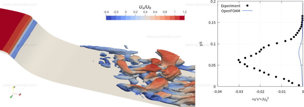
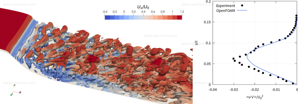
The new grey-area enhanced DES variants accelerate the RANS-LES transition in the early shear layer by reducing eddy viscosity locally. Regular subgrid-scale behaviour returns once the turbulence becomes fully developed. The following figures demonstrate the grey area effect for the recirculating flow downstream of a 2D wall-mounted hump. Significantly higher levels of resolved turbulence and better agreement with experiments are seen for the grey-area enhanced model.
Delayed emergence of resolved turbulence in the wake of a 2D hump caused by the grey area problem in standard DES formulation (SpalartAllmarasDDES). Isosurfaces of the Q criterion shaded with streamwise velocity (left) and resolved Reynolds shear stress profile (right).
Improved levels of resolved turbulence in the wake of a 2D hump for grey-area enhanced DES formulation (SpalartAllmarasDDES with activated option useSigma and DeltaOmegaTildeDelta filter definition). Isosurfaces of the Q criterion shaded with streamwise velocity (left) and resolved Reynolds shear stress profile (right).
The following turbulence modelling features are included in the v2212 release:
Grey-area enhanced \(\sigma\)-DDES formulation [1][3], SpalartAllmarasDDES and kOmegaSSTDDES with activated option useSigma, which is applicable to both Spalart-Allmaras and Menter SST-based DDES formulations;
Vorticity-adaptive filter definition, \(\tilde{\Delta}_\omega\)[4][5], DeltaOmegaTildeDelta, which is recommended for use in conjunction with the \(\sigma\)-DDES model; and
Shear-layer adaptive filter definition, \(\Delta_{SLA}\)[5], SLADelta, which achieves a similar effect to the combination of \(\sigma\)-DDES and \(\Delta_\omega\).
The grey-area enhanced DES model components were implemented by Upstream CFD GmbH and integrated into OpenFOAM in collaboration with OpenCFD Ltd with funding by Volkswagen AG.
Fuchs, M., Mockett, C., Sesterhenn, J., and Thiele, F. (2020). The grey-area enhanced sigma-DDES approach: Formulation review and application to complex test cases. In: Progress in Hybrid RANS-LES Modelling, Notes on Numerical Fluid Mechanics and Multidisciplinary Design 143, pp. 119-130, Springer, 2020.
Greenblatt, D., Paschal, K. B., Yao, C.-S., Harris, J., Schaeffler, N. W., & Washburn, A. E. (2006). Experimental Investigation of Separation Control Part 1: Baseline and Steady Suction. AIAA Journal, Vol. 44, No. 12, pp. 2820-2830, 2006.
Mockett, C., & Fuchs, M. (2017). Application of Alternative SGS Forms for Grey Area Mitigation. In Go4Hybrid, volume 134 of Notes on Numerical Fluid Mechanics and Multidisciplinary Design, Springer, 2017.
Mockett, C., Fuchs, M., Garbaruk, A.V., Shur, M.L., Spalart, P.R., Strelets, M.K., Thiele, F., & Travin, A.K. (2016). Two non-zonal approaches to accelerate RANS to LES transition of free shear layers in DES. In: Progress in Hybrid RANS-LES Modelling, Notes on Numerical Fluid Mechanics and Multidisciplinary Design 130, pp. 187-201, Springer, 2015.
Shur, M. L., Spalart, P. R., Strelets, M. K., & Travin, A. K. (2015). An enhanced version of DES with rapid transition from RANS to LES in separated flows. Flow, Turbulence and Combustion, 95, 709–737, 2015.
The inter-region heat transfer fvOption, effectivenessHeatExchangerSource has been renamed as heatExchangerSource, and extended to allow users to specify two new submodels:
effectivenessTable: the behaviour of the earlier effectivenessHeatExchangerSource; and
referenceTemperature: a model that uses a reference temperature - either a scalar or calculated from a two-dimensional interpolation table - to calculate the heat exchange.
A minimal example usage follows:
heatExchangerSource1
{
    type                    heatExchangerSource;

    // Option-1
    model                   effectivenessTable;

    // Option-2
    model                   referenceTemperature;
Multi-region cases can be challenging to assemble and operate. The new pureZoneMixture model can be used to simplify set-ups where regions differ only by the choice of thermophysical properties. Here, users can employ a single mesh region and select the thermophysical properties per cell zone, simplifying pre- and post-processing and potentially reducing run times.
Inter-zone coupling is treated implicitly using internal faces, or explicitly using boundary conditions. The internal face coupling is less flexible - there can be no additional resistance, e.g. shell conduction, or sources, e.g. radiation. For internal faces the effect of having discontinuous properties might be handled through, e.g. harmonic interpolation.
Zonal mixture
This takes a mixture setting for every cell zone. A typical constant/<region>/thermophysicalProperties for a solid region might contain
thermoType
{
    type            heSolidThermo;
    mixture         pureZoneMixture;
    transport       constIso;
    thermo          hConst;
    equationOfState rhoConst;
    specie          specie;
    energy          sensibleEnthalpy;
}

mixture
{
    leftSolid
    {
        specie
        {
            molWeight   50;
        }

        transport
        {
            kappa   80;
        }

        thermodynamics
        {
            Hf      0;
            Cp      450;
        }

        equationOfState
        {
            rho     8000;
        }
    }
    rightSolid
    {
        //- Start off from properties of cellZone leftSolid
        ${leftSolid}

        //- Selectively overwrite properties
        equationOfState
        {
            rho     2800;
        }
    }
}
Notes
The 'special' cellZone named none will match any unzoned cells;
pureZoneMixture can be applied to fluid regions, provided that they use the pureMixture, i.e. a non-reacting, single-component mixture;
Only the mixture properties can change;
you cannot have both fluid and solid in the same region;
pureZoneMixture will yield exactly the same results as pureMixture when the cell zones have the same mixture properties.
A new, optional, logFrequency entry has been added to the cloud solution input dictionary to reduce the amount of information the lagrangian models write to the log, e.g. in the /constant/*CloudProperties file, i.e.
solution
{
    active          true;
    coupled         false;
    transient       yes;
    cellValueSourceCorrection off;
    maxCo           0.3;

    logFrequency    3; // <--- NEW ENTRY

    ...
}
The value controls the number of carrier phase time steps that are performed between reporting lagrangian phase statistics, e.g.
Solving2-D cloud reactingCloud1
Cloud: reactingCloud1
    Current number of parcels       = 994
    Current mass in system          = 0.009735873844
    Linear momentum                 = (0.0001652067978 0.0001039875528 0)
   |Linear momentum|                = 0.0001952093676
    Linear kinetic energy           = 0.0001660812145
    Average particle per parcel     = 19.21387643
    Injector model1:
      - parcels added               = 994
      - mass introduced             = 0.01
    Parcel fate: system (number, mass)
      - escape                      = 0, 0
    Parcel fate: patch (walls|cyc.*) (number, mass)
      - escape                      = 0, 0
      - stick                       = 0, 0
    Parcel fate: patch (inlet|outlet) (number, mass)
      - escape                      = 0, 0
      - stick                       = 0, 0
    Temperature min/max             = 275.039299, 275.4193813
    Mass transfer phase change      = 0.000264126156
    Mass transfer devolatilisation  = 0
    Mass transfer surface reaction  = 0
The value is set to 1 by default to maintain backwards compatibility.
The finite area perturbedTemperatureDependentContactAngleForce has been renamed dynamicContactAngle and extended to include:
film-speed dependent contact-angle force calculation with stochastic perturbations; and
an additional force contribution acting against the motion of the contact line movement creating a hysteresis when the film thickness exceeds a critical film thickness.
A minimal example of this model can be seen below:
dynamicContactAngleForceCoeffs
{
    // Mandatory entries
    distribution    <subDict>;

    // Optional entries
    hCrit           <scalar>;  // Critical film height

    // Conditional entries

        // Option-1
        Utheta           <Function1<scalar>>;  // Contact angle vs film speed

        // Option-2
        Ttheta           <Function1<scalar>>;  // Contact angle vs film temperature

    // Inherited entries
    ...
}
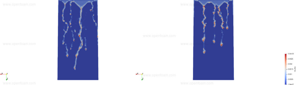
The illustration below shows a rivulet panel-flow case where the effects of using the critical film height and contact-angle vs film-speed entries are shown from left to right. The new implementation resulted in coalescence of rivulets on the right figure:
Meredith, K. V., Heather, A., De Vries, J., & Xin, Y. (2011). A numerical model for partially-wetted flow of thin liquid films. Computational Methods in Multiphase Flow VI, 70, 239.
Novák, M., Devaradja, R., Papper, J., & Černý, M. (2020). Efficient CFD methods for assessment of water management. In 20. Internationales Stuttgarter Symposium (pp. 151-170). Springer Vieweg, Wiesbaden.
The Brun film dripping model has been migrated from the finite volume film library to the finite area library. It is applied in the U/<filmPatch> velocityFilmShell definition for injection models, e.g.
The lagrangian surfaceFilmModel is responsible for transferring lagrangian parcels to finite-area and finite-volume film models. Users have a new parcelTypes entry, which describes the list of parcel type IDs interacting with a surface film. If the entry is omitted, all parcels participate.
surfaceFilmModel kinematicSurfaceFilm;

kinematicSurfaceFilmCoeffs
{
    interactionType absorb;

    // Optional list of participating parcel IDs
    parcelTypes     (10);
}
To set the parcel type by injector, injectorID entry can be used when specifying the injector models, e.g.
injectionModels
{
    model1
    {
        type            <injectionModelType>;

        // Optional injector ID
        // - if ommitted, parcels use '-1'
        injectorID      10;

        ...
    }
}
The new solidIsothermalReactionRate model provides isothermal reaction rates for solids alongside the solidArrheniusReactionRate model. A minimal example of this model is given below:
{
    // Mandatory entries
    C       <scalar>;  // Model constant
    Cp      <scalar>;  // Specific heat of solid material (assumed constant)
    Tpc     <scalar>;  // Phase change temperature
    Elat    <scalar>;  // Latent heat of phase change

    // Elat, the latent energy is defined in the present
    // implementation as a negative value (using the convention
    // endothermic process has negative enthalpy.)
}
W.H. Lee, A pressure iteration scheme for two-phase flow modeling, T.N. Veziroglu (Ed.), Multiphase Transport Fundamentals, Reactor Safety, Applications, vol. 1, Hemisphere Publishing, Washington, DC (1980).
Kharangate, C. R., & Mudawar, I. (2017). Review of computational studies on boiling and condensation. International Journal of Heat and Mass Transfer, 108, 1164-1196.