Overset dynamic mesh capabilities have been added to the base multiphase interPhaseChangeFoam and compressibleInterFoam applications, to create overInterPhaseChangeDyMFoam and overCompressibleInterDyMFoam.
The following video shows the twoSimpleRotors tutorial case using the new overInterPhaseChangeDyMFoam application.
The solar load model now allows time-dependent input as well as any other TimeFunction1 type input for direct solar irradiation, diffuse solar irradiation and spectral distribution.
The following example to produce a time-dependent load is taken from the simpleCarSolarPanel tutorial:
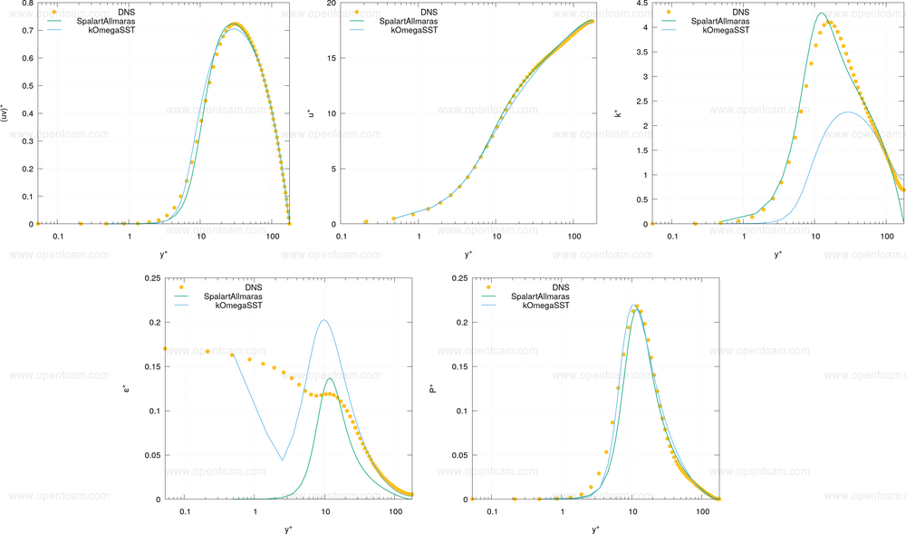
New estimation functions for the calculation of k, epsilon and omega fields for the Spalart-Allmaras turbulence model have been added. These enhancements enable various utilities, e.g. the turbulenceFields function object to return appropriate values, as opposed to the zero values in earlier releases.
A test case based on a direct-numerical simulation of a plane channel flow at $ \mathrm{Re}_\tau = 180 $ compares the prediction capabilities of these estimation functions in the SpalartAllmaras model to the kOmegaSST model, where k and omega exist internally.
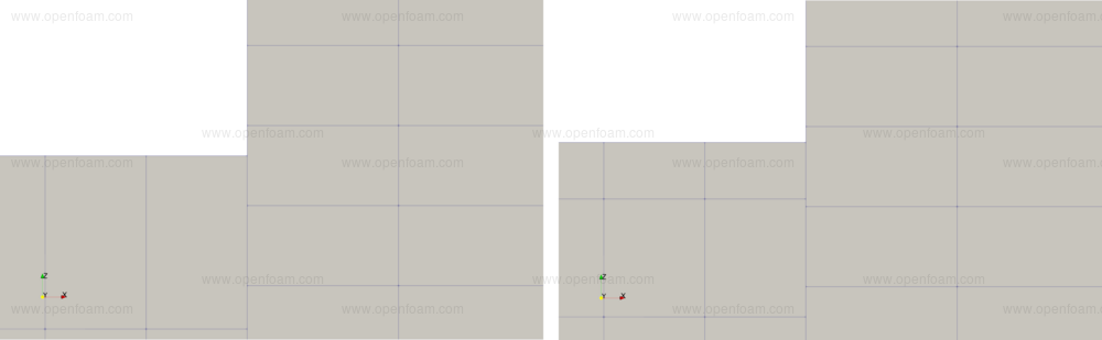
This is an extension of the dynamic layer addition/removal. It now supports adding/removing layers on cyclicACMI patches. This makes it much easier to handle partial obstructions.
In below pictures (before and after the addition of a layer of cells) the obstruction (on the left, white background) slides along a cyclicACMI. The cyclicACMI takes care of connecting the left cells to the cells on the right using face-area weighted interpolation.
The new improvement in the RanzMarshall model generalises the Nusselt number correlation expression by allowing users to input custom correlation coefficients.
A minimal example is shown below:
subModels
{
    RanzMarshallCoeffs
    {
        // a + b Re^m Pr^n
        a 2.0;
        b 0.6;
        m 0.5;
        n 0.6666;
    }
}
Dynamic overset mesh functionality was made compatible with multiple motion solvers in an earlier release, enabling multiple, overlapping domains.
This release introduces further enhancements:
Added zoneMotion to rigidBodyMotion: This option is convenient to select a subset of cells which are transformed by the displacement of the rigidBodyMotion solver.
Introduced proportional–integral–derivative (PID) control to the prescribedRotation restraint: Numerical robustness of the prescribedRotation restraint has been improved by a new PID system to obtain the desired angular momentum. In the example input dictionary below, p is the proportional corrector, d the differential corrector, i the integral corrector, and relax is the relaxation factor:
propellerRotation
{
    type                    prescribedRotation;
    body                    propeller;
    referenceOrientation    (1 0 0 0 1 0 0 0 1);
    axis                    (1 0 0);

    relax                   0.2;
    p                       0.001;
    d                       0.01;
    i                       0;
    omega                   table
    (
        (0       (0 0 0))
        (0.1     (149 0 0))
        (0.5     (628 0 0))
    );
}
drivenLinearMotion can be used in six-Dof and rigid-body solvers: drivenLinearMotion is a rigid body motion solver that allows to 'follow' a given centre of mass. This enables the background mesh to move to accommodate the inset rigid body mesh, i.e. the floating object. This avoids the need to employ large background meshes when the displacement of the inset object is larger than the background domain.
The rigidBodyMotion stores the centre of gravity displacement (cOfGdisplacement CofG) of its body identifier (bodyIdCofG 1), and drivenLinearMotion reads the entry cOfGdisplacement.
The makeFaMesh utility and corresponding finiteArea infrastructure has been updated and improved to create finite-area meshes in parallel. A typical use case would be when the volume mesh has been created in parallel, e.g. with snappyHexMesh, and a region with a finite-area mesh is needed. The updated version now supports creation of a finite-area mesh in parallel, and simultaneously decomposes finite area fields.
The definition of the finite-area mesh, i.e. faMeshDefinition, is now more flexible, requires fewer mandatory inputs, and handles some common corner cases.
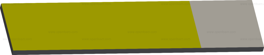
In the example geometry, the original mesh has been split into eight sub-domains.
finiteArea case example
This particular decomposition has been chosen as one of the corner cases, since the finite-area region is only present on some of the domains. Although the finite-area terminates exactly on the processor-processor boundary, the makeFaMesh routine correctly defines the physical outflow boundary and the internal decomposition of the initial fields is correctly handled.
In addition to streamlining case set-ups, these new changes allow on-the-fly definition of finite-area regions during the calculation which should be part of a future release.