
v2112: New and improved numerics
TOP
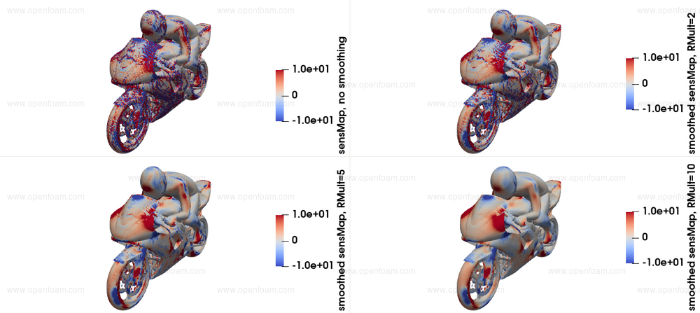
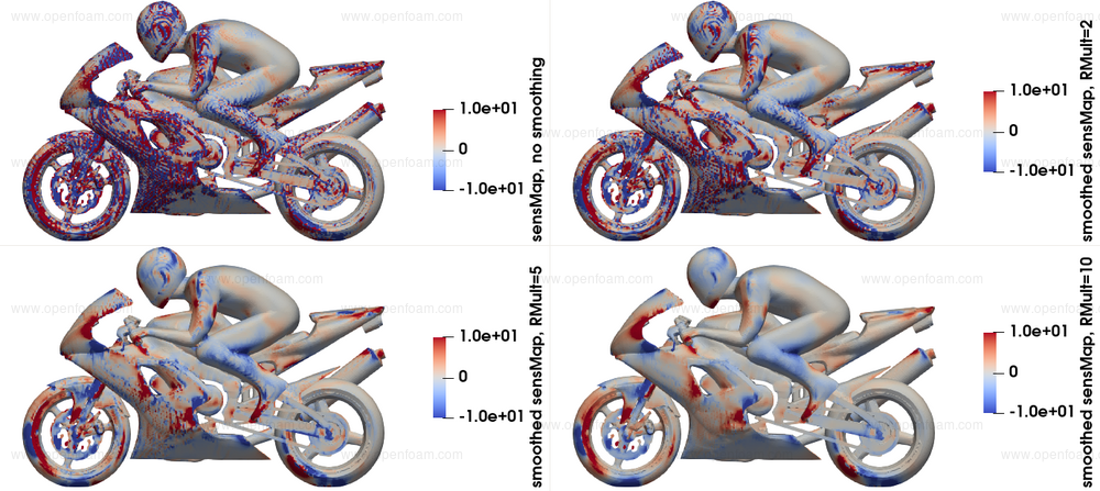
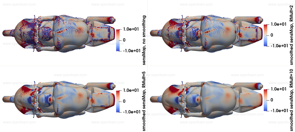
Adjoint-based sensitivity maps can now be optionally smoothed using a Laplace-Beltrami operator.
When computing sensitivity maps on surface meshes generated from industrial geometries, the outcome might appear noisy, especially if a volume-to-surface approach is used for meshing, e.g. as used by snappyHexMesh. Even though the sensitivity map is technically correct, the noisy patterns that appear might make the extraction of useful information challenging. This new feature facilitates the interpretation of the sensitivity map in such cases.
Details of new models
The sensitivity map can be smoothed using a Laplace-Beltrami operator of the form
\[ \tilde{m} - \frac{\partial}{\partial x_j}\left[R^2\frac{\partial \tilde{m}}{\partial x_j}\right] = m \]
where $\tilde{m}$ is the smoothed sensitivity map, $m$ is the original sensitivity map and $R$ a smoothing radius. The latter is computed as a multiple of the average 'length' of the boundary faces, if not provided by the user explicitly.
This equation is solved on the part of the surface mesh defined by the patches on which the sensitivity map is computed, using finiteArea methods.
If a finite area mesh is provided, it will be used; otherwise it is created on-the-fly based on either an faMeshDefinition dictionary in the system directory, or constructed internally based on the sensitivity patches.
From an optimisation point of view, this smoothing can alternatively be seen as computing the sensitivity derivatives $\frac{\delta J}{\delta b_i}$ of the objective function $J$ w.r.t. a different set of design variables $b_i, i\in[1,N]$, defined as
\[ x_i = x_i^{init} + \tilde{b_i} \\ \tilde{b_i} - \frac{\partial}{\partial x_j}\left[R^2\frac{\partial \tilde{b_i}}{\partial x_j}\right] = b_i \]
where $x_i$ are the coordinates of the updated geometry and $\tilde{b_i}$ a smooth displacement field. In other words, no loss of accuracy is incurred by the smoothing; instead, sensitivities are computed w.r.t. a different set of design variables.
Examples
An example of a noisy sensitivity map and its smoothed variants using different $R$ values is presented below, taken from the updated motorBike tutorial:
Usage
To enable the smoothing, the smoothSensitivities boolean should be set to true, along with some optional entries.
sensitivities
{
    type                 surfacePoints;
    patches              (motorBikeGroup);
    includeSurfaceArea   false;
    smoothSensitivities  true;
    meanRadiusMultiplier 10;    // Optional, defaults to 10. Controls the smoothing radius
    iters                2000;  // Optional, defaults to 500
}
Since the Laplace-Beltrami equation is solved using the finiteArea framework, faSchemes and faSolution files should be present under the system directory.
The smoothed sensitivity map is written to the 'smoothedSurfaceSens + adjointSolverName + sensitivityFormulation' file, under the current time-step.
Source code
Tutorial
Attribution
- The software was developed by PCOpt/NTUA and FOSS GP
References
- The notion of sensitivity smoothing using a Laplace-Beltrami operator was used throught the seminal works of Antony Jameson. A reference can be found in: Vassberg J. C., Jameson A. (2006). Aerodynamic Shape Optimization Part I: Theoretical Background. VKI Lecture Series, Introduction to Optimization and Multidisciplinary Design, Brussels, Belgium, 8 March, 2006.
TOP
In this release the cyclicPeriodicAMI coupled patch numerics have been made consistent with the geometry matching. The cyclicPeriodicAMI is a variant of cyclicAMI that automatically repeats the source geometry to cover all of the target geometry. This repetition can either be planar or cylindrical; the latter is particularly useful for turbine applications. In earlier releases the cylindrical (not planar) repetition case transformed the geometry, but not the corresponding fields.
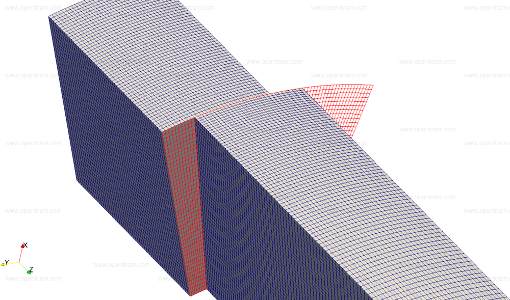
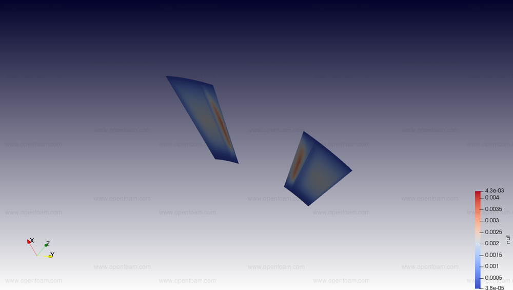
As an example, the following image shows a typical geometry where the source and target geometry are not identical, requiring multiple transformations of the source geometry to cover the target geometry.
Not applying the corresponding transformation when interpolating vector- or tensor-fields causes artefacts across the repetitions, e.g. the turbulent viscosity field clearly shows non-physical behaviour:
This behaviour is not directly visible in axial components of fields, e.g. the flux is not directly affected, nor scalar fields, e.g. pressure. The error increases with the difference in transformation angle between source and target.
In this version the underlying cyclicAMI interpolation automatically detects
- presence of a periodic patch with a rotational transformation
- vector or tensor fields
and converts all variables into the coordinate system of the periodic patch before interpolation and reverse interpolates the result afterwards. This assures a consistent behaviour across multiple repetitions of the geometry.
Caveats:
- It assumes all non-scalar fields on the patches are in global coordinates. This is almost always the case since all discretisation assumes the same.
- It only handles 'normal' fields, not e.g. wall distance information that use the meshWave method.
- There is a small inconsistency due to the geometry (face centres, area weights) being calculated in Cartesian coordinates whereas the interpolation is performed using cylindrical coordinates. This error is of similar order to using faceted discretisation of cylindrical geometries.
Tutorials
Source code
TOP
All under-relaxation factors in the system/fvSolution dictionary are now Function1s, permitting time dependent profiles, e.g. using the table method:
relaxationFactors
{
    equations
    {
        // Ramp the relaxation factors
        "(U|e|k|epsilon).*" table ((0 0.4) (0.5 0.7));
    }
}
This will ramp the relaxation factor from 0.4 to 0.7 over the time interval 0 to 0.5s.
Tutorials
Source code
TOP
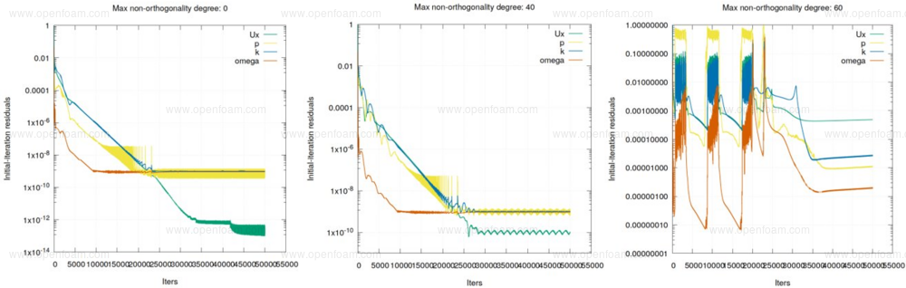
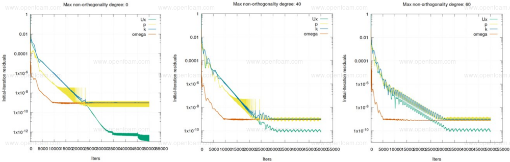
A new Laplacian scheme, relaxedNonOrthoLaplacian, and a new surface-normal gradient scheme, relaxedSnGrad, improve the numerical stability of cases with high non-orthogonality via changes in the handling of the diffusion operator. Benefits of these new schemes are demonstrated below using a new high-fidelity setup, where the residuals are shown as a function of face non-orthogonality angle for a base, and control-variable relaxedSnGrad simulation, respectively:
Source code
- $FOAM_SRC/finiteVolume/finiteVolume/laplacianSchemes/relaxedNonOrthoGaussLaplacianScheme
- $FOAM_SRC/finiteVolume/finiteVolume/snGradSchemes/relaxedSnGrad
Tutorial
Merge request
TOP
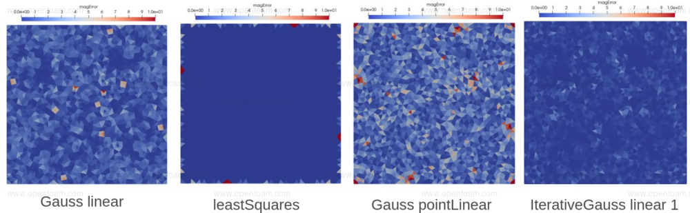
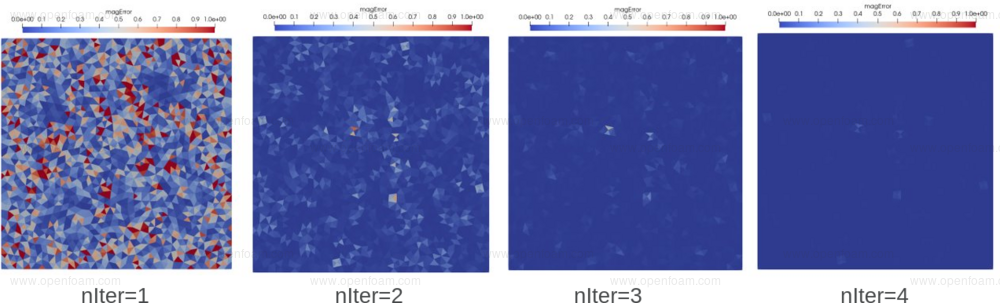
A new Gauss-Green gradient scheme, iterativeGauss, offers improved performance for meshes with non-zero face skewness by adding an outer loop around the Gauss-Green gradient scheme and skew-correction vector computations.
The main benefit of this scheme is demonstrated below using a manufactured solution that shows the level of skewness-related errors:
The scheme allows a user-specified number of outer iterations, which can reduce the level of errors in exchange for increased computational cost:
Source code
Tutorial
Merge request
TOP
This release includes a new implicit treatment for coupled patches, which operates by substituting cyclic or mapped boundary faces with virtual internal faces.
Additional pre-processing is applied during matrix assembly to determine which faces are internal, and where to insert new connections between coupled patch cells. In the case of collocated patches, i.e. one-to-one face mapping, each new internal face is connected to two cells. However, AMI and ACMI patches have one-to-many face connectivity; here, the number of new internal faces corresponds to the number of connections.
Usage
The new behaviour is activated using the keyword useImplicit; this is supported by cyclic, cyclicAMI, cyclicACMI and mapped boundary conditions, e.g.
boundaryField
{
    AMI1
    {
        type            cyclicAMI;
        useImplicit     true;
    }

    AMI2
    {
        type            cyclicAMI;
        useImplicit     true;
    }
}
This flag can be specified per coupled patch pair, per field, i.e. it is possible to set the useImplicit option for pressure but not for turbulence fields on the same cyclic patches. Currently there is a limitation regarding parallel running which requires AMI or ACMI patches to reside on the same processor. This can be achieved using a constrained decomposition, e.g. in the decomposeParDict:
numberOfSubdomains  3;
method  scotch;

constraints
{
    faces
    {
        type    preserveFaceZones;
        zones   (f1 f2);
        enabled true;
    }
}
Note: when using GAMG solver the recommended setup is:
solver              GAMG;
...
cacheAgglomeration  false;
agglomerator        assembledFaceAreaPair;
....
In solvers where the option correctPhi is available, e.g. pimpleFoam, the implicit option cannot be used for the pcorr variable since it is created on-the-fly and would destroy the flux consistency.
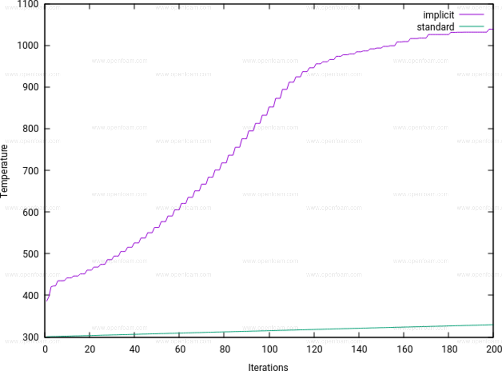
An example usage for the new option is to solve for a single temperature field in multi-region conjugate heat transfer (CHT) cases. This produces a closer coupling between disconnected regions, yielding an energy equation that is easier to converge compared to using mapped patches. Applying this approach is particularly beneficial for quasi-steady flow conditions and the temperature field requires inner loops across multiple solid/fluid regions. The image below compares the temperature time histories for the cpuCabinet tutorial when running with, and without, the implicit option:
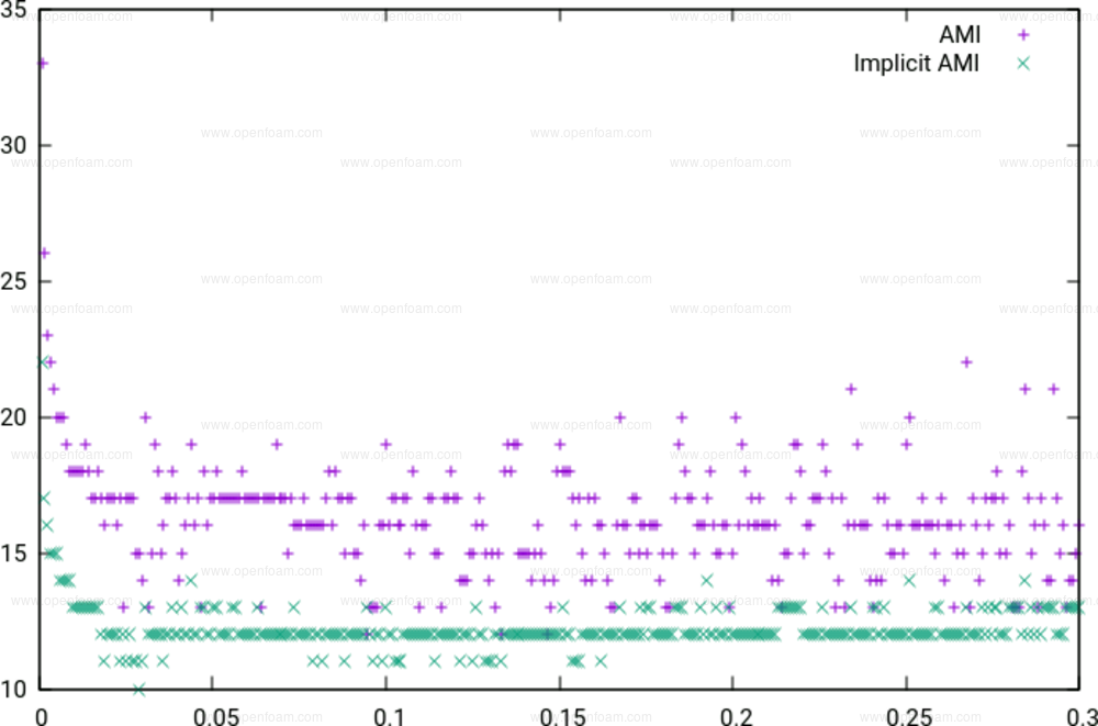
Advantages have also been observed for single phase cases, particularly if the coupled patches play an important role in determining the flow pattern and convergence rate. The following image shows the number of pressure equation iterations for a 2D lift case, evaluated using the pimpleFoam solver, where two AMI interfaces are located along the complete length of the domain:
Tutorials