2.2 Flow around a cylinder
Tutorial path:
In this example we shall investigate potential flow around a cylinder using thepotentialFoam solver. This example introduces the following OpenFOAM features:
- non-orthogonal meshes;
- generating an analytical solution to a problem in OpenFOAM;
- use of a dynamic code to generate the block vertices;
- use of a coded function object to compare results against the analytical solution.
2.2.1 Problem specification
The problem is defined as follows:
- Solution domain
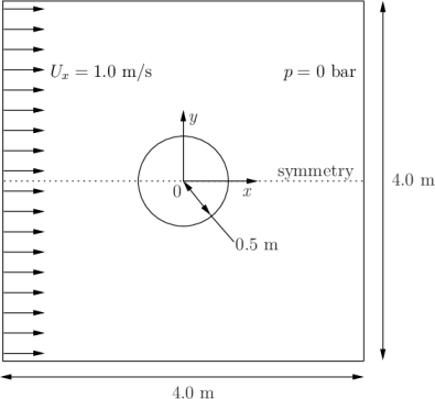
- The domain is 2 dimensional and consists of a square domain with
a cylinder collocated with the centre of the square as shown in Figure 2.15.
- Governing equations
- Boundary conditions
-
- Inlet (left) with fixed velocity
 .
.
- Outlet (right) with a fixed pressure
 .
.
- No-slip wall (bottom);
- Symmetry plane (top).
- Inlet (left) with fixed velocity
- Initial conditions
 ,
,  — required in OpenFOAM
input files but not necessary for the solution since the problem is
steady-state.
— required in OpenFOAM
input files but not necessary for the solution since the problem is
steady-state.
- Solver name
- potentialFoam: a potential flow code, i.e. assumes the flow is incompressible, steady, irrotational, inviscid and it ignores gravity.
- Case name
- cylinder case located in the $FOAM_TUTORIALS/basic/potentialFoam directory.


2.2.2 Note on potentialFoam
potentialFoam is a useful solver to validate OpenFOAM since the assumptions of
potential flow are such that an analytical solution exists for cases whose
geometries are relatively simple. In this example of flow around a cylinder an
analytical solution exists with which we can compare our numerical solution.
potentialFoam can also be run more like a utility to provide a (reasonably)
conservative initial  field for a problem. When running certain cases, this can
useful for avoiding instabilities due to the initial field being unstable. In short,
potentialFoam creates a conservative field from a non-conservative initial field
supplied by the user.
field for a problem. When running certain cases, this can
useful for avoiding instabilities due to the initial field being unstable. In short,
potentialFoam creates a conservative field from a non-conservative initial field
supplied by the user.
2.2.3 Mesh generation
Mesh generation using blockMesh has been described in tutorials in the User
Guide. In this case, the mesh consists of  blocks as shown in Figure 2.16.
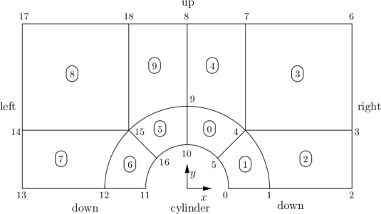
Remember that all meshes are treated as 3 dimensional in OpenFOAM. If we
wish to solve a 2 dimensional problem, we must describe a 3 dimensional mesh
that is only one cell thick in the third direction that is not solved. In Figure 2.16
we show only the back plane of the geometry, along  , in which the
vertex numbers are numbered 0-18. The other 19 vertices in the front plane,
, in which the
vertex numbers are numbered 0-18. The other 19 vertices in the front plane,
 , are numbered in the same order as the back plane, as shown in the
mesh description file below:
, are numbered in the same order as the back plane, as shown in the
mesh description file below:
1/*--------------------------------*- C++ -*----------------------------------*\
2| ========= | |
3| \\ / F ield | OpenFOAM: The Open Source CFD Toolbox |
4| \\ / O peration | Version: v2006 |
5| \\ / A nd | Website: www.openfoam.com |
6| \\/ M anipulation | |
7\*---------------------------------------------------------------------------*/
8FoamFile
9{
10 version 2.0;
11 format ascii;
12 class dictionary;
13 object blockMeshDict;
14}
15// * * * * * * * * * * * * * * * * * * * * * * * * * * * * * * * * * * * * * //
16
17scale 1;
18
19vertices #codeStream
20{
21 codeInclude
22 #{
23 #include "pointField.H"
24 #};
25
26 code
27 #{
28 pointField points(19);
29 points[0] = point(0.5, 0, -0.5);
30 points[1] = point(1, 0, -0.5);
31 points[2] = point(2, 0, -0.5);
32 points[3] = point(2, 0.707107, -0.5);
33 points[4] = point(0.707107, 0.707107, -0.5);
34 points[5] = point(0.353553, 0.353553, -0.5);
35 points[6] = point(2, 2, -0.5);
36 points[7] = point(0.707107, 2, -0.5);
37 points[8] = point(0, 2, -0.5);
38 points[9] = point(0, 1, -0.5);
39 points[10] = point(0, 0.5, -0.5);
40 points[11] = point(-0.5, 0, -0.5);
41 points[12] = point(-1, 0, -0.5);
42 points[13] = point(-2, 0, -0.5);
43 points[14] = point(-2, 0.707107, -0.5);
44 points[15] = point(-0.707107, 0.707107, -0.5);
45 points[16] = point(-0.353553, 0.353553, -0.5);
46 points[17] = point(-2, 2, -0.5);
47 points[18] = point(-0.707107, 2, -0.5);
48
49 // Duplicate z points
50 label sz = points.size();
51 points.setSize(2*sz);
52 for (label i = 0; i < sz; i++)
53 {
54 const point& pt = points[i];
55 points[i+sz] = point(pt.x(), pt.y(), -pt.z());
56 }
57
58 os << points;
59 #};
60};
61
62
63blocks
64(
65 hex (5 4 9 10 24 23 28 29) (10 10 1) simpleGrading (1 1 1)
66 hex (0 1 4 5 19 20 23 24) (10 10 1) simpleGrading (1 1 1)
67 hex (1 2 3 4 20 21 22 23) (20 10 1) simpleGrading (1 1 1)
68 hex (4 3 6 7 23 22 25 26) (20 20 1) simpleGrading (1 1 1)
69 hex (9 4 7 8 28 23 26 27) (10 20 1) simpleGrading (1 1 1)
70 hex (15 16 10 9 34 35 29 28) (10 10 1) simpleGrading (1 1 1)
71 hex (12 11 16 15 31 30 35 34) (10 10 1) simpleGrading (1 1 1)
72 hex (13 12 15 14 32 31 34 33) (20 10 1) simpleGrading (1 1 1)
73 hex (14 15 18 17 33 34 37 36) (20 20 1) simpleGrading (1 1 1)
74 hex (15 9 8 18 34 28 27 37) (10 20 1) simpleGrading (1 1 1)
75);
76
77edges
78(
79 arc 0 5 (0.469846 0.17101 -0.5)
80 arc 5 10 (0.17101 0.469846 -0.5)
81 arc 1 4 (0.939693 0.34202 -0.5)
82 arc 4 9 (0.34202 0.939693 -0.5)
83 arc 19 24 (0.469846 0.17101 0.5)
84 arc 24 29 (0.17101 0.469846 0.5)
85 arc 20 23 (0.939693 0.34202 0.5)
86 arc 23 28 (0.34202 0.939693 0.5)
87 arc 11 16 (-0.469846 0.17101 -0.5)
88 arc 16 10 (-0.17101 0.469846 -0.5)
89 arc 12 15 (-0.939693 0.34202 -0.5)
90 arc 15 9 (-0.34202 0.939693 -0.5)
91 arc 30 35 (-0.469846 0.17101 0.5)
92 arc 35 29 (-0.17101 0.469846 0.5)
93 arc 31 34 (-0.939693 0.34202 0.5)
94 arc 34 28 (-0.34202 0.939693 0.5)
95);
96
97boundary
98(
99 down
100 {
101 type symmetryPlane;
102 faces
103 (
104 (0 1 20 19)
105 (1 2 21 20)
106 (12 11 30 31)
107 (13 12 31 32)
108 );
109 }
110 right
111 {
112 type patch;
113 faces
114 (
115 (2 3 22 21)
116 (3 6 25 22)
117 );
118 }
119 up
120 {
121 type symmetryPlane;
122 faces
123 (
124 (7 8 27 26)
125 (6 7 26 25)
126 (8 18 37 27)
127 (18 17 36 37)
128 );
129 }
130 left
131 {
132 type patch;
133 faces
134 (
135 (14 13 32 33)
136 (17 14 33 36)
137 );
138 }
139 cylinder
140 {
141 type symmetry;
142 faces
143 (
144 (10 5 24 29)
145 (5 0 19 24)
146 (16 10 29 35)
147 (11 16 35 30)
148 );
149 }
150);
151
152mergePatchPairs
153(
154);
155
156// ************************************************************************* //
2.2.4 Boundary conditions and initial fields
Edit the case files to set the boundary conditions in accordance with
the problem description in Figure 2.15, i.e. the left boundary should
be an Inlet, the right boundary should be an Outlet and the down and
cylinder boundaries should be symmetryPlane. The top boundary conditions
is chosen so that we can make the most genuine comparison with our
analytical solution which uses the assumption that the domain is infinite in
the  direction. The result is that the normal gradient of
  is small
along a plane coinciding with our boundary. We therefore impose the
condition that the normal component is zero, i.e. specify the boundary as a
symmetryPlane, thereby ensuring that the comparison with the analytical is
reasonable.
is small
along a plane coinciding with our boundary. We therefore impose the
condition that the normal component is zero, i.e. specify the boundary as a
symmetryPlane, thereby ensuring that the comparison with the analytical is
reasonable.
2.2.5 Running the case
No fluid properties need be specified in this problem since the flow is assumed to be incompressible and inviscid. In the system subdirectory, the controlDict specifies the control parameters for the run. Note that since we assume steady flow, we only run for 1 time step:
1/*--------------------------------*- C++ -*----------------------------------*\
2| ========= | |
3| \\ / F ield | OpenFOAM: The Open Source CFD Toolbox |
4| \\ / O peration | Version: v2006 |
5| \\ / A nd | Website: www.openfoam.com |
6| \\/ M anipulation | |
7\*---------------------------------------------------------------------------*/
8FoamFile
9{
10 version 2.0;
11 format ascii;
12 class dictionary;
13 location "system";
14 object controlDict;
15}
16// * * * * * * * * * * * * * * * * * * * * * * * * * * * * * * * * * * * * * //
17
18application potentialFoam;
19
20startFrom latestTime;
21
22startTime 0;
23
24stopAt nextWrite;
25
26endTime 1;
27
28deltaT 1;
29
30writeControl timeStep;
31
32writeInterval 1;
33
34purgeWrite 0;
35
36writeFormat ascii;
37
38writePrecision 6;
39
40writeCompression off;
41
42timeFormat general;
43
44timePrecision 6;
45
46runTimeModifiable true;
47
48functions
49{
50 error
51 {
52 name error;
53 type coded;
54 libs (utilityFunctionObjects);
55
56 codeEnd
57 #{
58 // Lookup U
59 Info<< "Looking up field U\n" << endl;
60 const volVectorField& U = mesh().lookupObject<volVectorField>("U");
61
62 Info<< "Reading inlet velocity uInfX\n" << endl;
63
64 scalar ULeft = 0.0;
65 label leftI = mesh().boundaryMesh().findPatchID("left");
66 const fvPatchVectorField& fvp = U.boundaryField()[leftI];
67 if (fvp.size())
68 {
69 ULeft = fvp[0].x();
70 }
71 reduce(ULeft, maxOp<scalar>());
72
73 dimensionedScalar uInfX("uInfx", dimVelocity, ULeft);
74
75 Info<< "U at inlet = " << uInfX.value() << " m/s" << endl;
76
77
78 scalar magCylinder = 0.0;
79 label cylI = mesh().boundaryMesh().findPatchID("cylinder");
80 const fvPatchVectorField& cylFvp = mesh().C().boundaryField()[cylI];
81 if (cylFvp.size())
82 {
83 magCylinder = mag(cylFvp[0]);
84 }
85 reduce(magCylinder, maxOp<scalar>());
86
87 dimensionedScalar radius("radius", dimLength, magCylinder);
88
89 Info<< "Cylinder radius = " << radius.value() << " m" << endl;
90
91 volVectorField UA
92 (
93 IOobject
94 (
95 "UA",
96 mesh().time().timeName(),
97 U.mesh(),
98 IOobject::NO_READ,
99 IOobject::AUTO_WRITE
100 ),
101 U
102 );
103
104 Info<< "\nEvaluating analytical solution" << endl;
105
106 const volVectorField& centres = UA.mesh().C();
107 volScalarField magCentres(mag(centres));
108 volScalarField theta(acos((centres & vector(1,0,0))/magCentres));
109
110 volVectorField cs2theta
111 (
112 cos(2*theta)*vector(1,0,0)
113 + sin(2*theta)*vector(0,1,0)
114 );
115
116 UA = uInfX*(dimensionedVector(vector(1,0,0))
117 - pow((radius/magCentres),2)*cs2theta);
118
119 // Force writing of UA (since time has not changed)
120 UA.write();
121
122 volScalarField error("error", mag(U-UA)/mag(UA));
123
124 Info<<"Writing relative error in U to " << error.objectPath()
125 << endl;
126
127 error.write();
128 #};
129 }
130}
131
132
133// ************************************************************************* //
potentialFoam executes an iterative loop around the pressure equation which it
solves in order that explicit terms relating to non-orthogonal correction in
the Laplacian term may be updated in successive iterations. The number of
iterations around the pressure equation is controlled by the
nNonOrthogonalCorrectors keyword in the fvSolution dictionary. In the
first instance we can set nNonOrthogonalCorrectors to 0 so that no loops
are performed, i.e. the pressure equation is solved once, and there is no
non-orthogonal correction. The solution is shown in Figure 2.17(a) (at
 , when the steady-state simulation is complete).
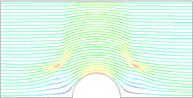
(a) With no non-orthogonal correction |
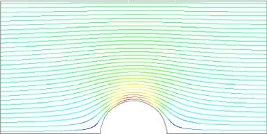
(b) With non-orthogonal correction |
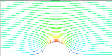
(c) Analytical solution |
Figure 2.17: Streamlines of potential flow
We expect the solution to show smooth streamlines passing across the domain as in the analytical solution in Figure 2.17(c), yet there is clearly some error in the regions where there is high non-orthogonality in the mesh, e.g. at the join of blocks 0, 1 and 3. The case can be run a second time with some non-orthogonal correction by setting nNonOrthogonalCorrectors to 3. The solution shows smooth streamlines with no significant error due to non-orthogonality as shown in Figure 2.17(b).