
2.1 Lid-driven cavity flow
Tutorial path:
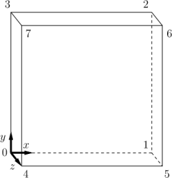
This tutorial will describe how to pre-process, run and post-process a case involving
isothermal, incompressible flow in a two-dimensional square domain. The
geometry is shown in Figure 2.1 in which all the boundaries of the square are
walls. The top wall moves in the  -direction at a speed of 1 m/s while the
other 3 are stationary. Initially, the flow will be assumed laminar and
will be solved on a uniform mesh using the icoFoam solver for laminar,
isothermal, incompressible flow. During the course of the tutorial, the effect of
increased mesh resolution and mesh grading towards the walls will be
investigated. Finally, the flow Reynolds number will be increased and the
pisoFoam solver will be used for turbulent, isothermal, incompressible flow.
-direction at a speed of 1 m/s while the
other 3 are stationary. Initially, the flow will be assumed laminar and
will be solved on a uniform mesh using the icoFoam solver for laminar,
isothermal, incompressible flow. During the course of the tutorial, the effect of
increased mesh resolution and mesh grading towards the walls will be
investigated. Finally, the flow Reynolds number will be increased and the
pisoFoam solver will be used for turbulent, isothermal, incompressible flow.

2.1.1 Pre-processing
In preparation of editing case files and running the first cavity case, the user should change to the case directory
cd $FOAM_RUN/tutorials/incompressible/icoFoam/cavity/cavity
2.1.1.1 Mesh generation
OpenFOAM always operates in a 3 dimensional Cartesian coordinate system and all geometries are generated in 3 dimensions. OpenFOAM solves the case in 3 dimensions by default but can be instructed to solve in 2 dimensions by specifying a ‘special’ empty boundary condition on boundaries normal to the (3rd) dimension for which no solution is required. Here, the mesh must be 1 cell layer thick, and the empty patches planar.
The cavity domain consists of a square of side length  in the
  -
- plane. A uniform mesh of 20 by 20 cells will be used initially. The block structure
is shown in Figure 2.2.
plane. A uniform mesh of 20 by 20 cells will be used initially. The block structure
is shown in Figure 2.2.
The blockMesh mesh generator supplied with OpenFOAM generates meshes from a description specified in an input dictionary, blockMeshDict located in the system directory for a given case. The blockMeshDict entries for this case are as follows:
1/*--------------------------------*- C++ -*----------------------------------*\
2| ========= | |
3| \\ / F ield | OpenFOAM: The Open Source CFD Toolbox |
4| \\ / O peration | Version: v2006 |
5| \\ / A nd | Website: www.openfoam.com |
6| \\/ M anipulation | |
7\*---------------------------------------------------------------------------*/
8FoamFile
9{
10 version 2.0;
11 format ascii;
12 class dictionary;
13 object blockMeshDict;
14}
15// * * * * * * * * * * * * * * * * * * * * * * * * * * * * * * * * * * * * * //
16
17scale 0.1;
18
19vertices
20(
21 (0 0 0)
22 (1 0 0)
23 (1 1 0)
24 (0 1 0)
25 (0 0 0.1)
26 (1 0 0.1)
27 (1 1 0.1)
28 (0 1 0.1)
29);
30
31blocks
32(
33 hex (0 1 2 3 4 5 6 7) (20 20 1) simpleGrading (1 1 1)
34);
35
36edges
37(
38);
39
40boundary
41(
42 movingWall
43 {
44 type wall;
45 faces
46 (
47 (3 7 6 2)
48 );
49 }
50 fixedWalls
51 {
52 type wall;
53 faces
54 (
55 (0 4 7 3)
56 (2 6 5 1)
57 (1 5 4 0)
58 );
59 }
60 frontAndBack
61 {
62 type empty;
63 faces
64 (
65 (0 3 2 1)
66 (4 5 6 7)
67 );
68 }
69);
70
71mergePatchPairs
72(
73);
74
75// ************************************************************************* //
The file first contains header information in the form of a banner (lines 1-7), then file information contained in a FoamFile sub-dictionary, delimited by curly braces ({…}).
For the remainder of the manual:
For the sake of clarity and to save space, file headers, including the banner
and FoamFile sub-dictionary, will be removed from verbatim quoting of case
files
The file first specifies the list of coordinates representing the block vertices; These are in arbitrary units, and can be scaled to the real problem dimensions using the scale entry, e.g.
scale 0.1;
The mesh is generated by running blockMesh on this blockMeshDict file. From within the case directory, this is done, simply by typing in the terminal:
blockMesh
2.1.1.2 Boundary and initial conditions
Once the mesh generation is complete, the user can look at this initial fields set
up for this case. The case is set up to start at time  s, so the initial field
data is stored in a 0 sub-directory of the cavity directory. The 0 sub-directory
contains 2 files, p and U, one for each of the pressure (
s, so the initial field
data is stored in a 0 sub-directory of the cavity directory. The 0 sub-directory
contains 2 files, p and U, one for each of the pressure ( ) and velocity (
 ) fields
whose initial values and boundary conditions must be set. Let us examine file
p:
) fields
whose initial values and boundary conditions must be set. Let us examine file
p:
17dimensions [0 2 -2 0 0 0 0];
18
19internalField uniform 0;
20
21boundaryField
22{
23 movingWall
24 {
25 type zeroGradient;
26 }
27
28 fixedWalls
29 {
30 type zeroGradient;
31 }
32
33 frontAndBack
34 {
35 type empty;
36 }
37}
38
39// ************************************************************************* //
18
19internalField uniform 0;
20
21boundaryField
22{
23 movingWall
24 {
25 type zeroGradient;
26 }
27
28 fixedWalls
29 {
30 type zeroGradient;
31 }
32
33 frontAndBack
34 {
35 type empty;
36 }
37}
38
39// ************************************************************************* //
There are 3 principal entries in field data files:
- dimensions
- specifies the dimensions of the field, here kinematic pressure,
i.e.
 (see User Guide section ?? for more information);
- internalField
- the internal field data which can be uniform, described by a single value; or nonuniform, where all the values of the field must be specified (see User Guide section ?? for more information);
- boundaryField
- the boundary field data that includes boundary conditions and data for all the boundary patches (see User Guide section ?? for more information).
For this case cavity, the boundary consists of walls only, split into 2 patches named: (1) fixedWalls for the fixed sides and base of the cavity; (2) movingWall for the moving top of the cavity. As walls, both are given a zeroGradient boundary condition for p, meaning “the normal gradient of pressure is zero”. The frontAndBack patch represents the front and back planes of the 2D case and therefore must be set as empty.
In this case, as in most we encounter, the initial fields are set to be uniform. Here the pressure is kinematic, and as an incompressible case, its absolute value is not relevant, so is set to uniform 0 for convenience.
The user can similarly examine the velocity field in the 0/U file. The dimensions are those expected for velocity, the internal field is initialised as uniform zero, which in the case of velocity must be expressed by 3 vector components, i.e.uniform (0 0 0) (see User Guide section ?? for more information).
The boundary field for velocity requires the same boundary condition for the
frontAndBack patch. The other patches are walls: a no-slip condition is
assumed on the fixedWalls, hence a fixedValue condition with a value of
uniform (0 0 0). The top surface moves at a speed of 1 m/s in the
 -direction so requires a fixedValue condition also but with uniform (1 0
0).
-direction so requires a fixedValue condition also but with uniform (1 0
0).
2.1.1.3 Physical properties
The physical properties for the case are stored in dictionaries whose names are
given the suffix …Properties, located in the constant directory tree. For an
icoFoam case, the only property that must be specified is the kinematic
viscosity which is stored from the transportProperties dictionary. The user
can check that the kinematic viscosity is set correctly by opening the
transportProperties dictionary to view/edit its entries. The keyword for
kinematic viscosity is nu, the phonetic label for the Greek symbol  by which it is represented in equations. Initially this case will be run
with a Reynolds number of 10, where the Reynolds number is defined
as:
by which it is represented in equations. Initially this case will be run
with a Reynolds number of 10, where the Reynolds number is defined
as:
 | (2.1) |
where  and
and  are the characteristic length and velocity respectively and
  is the kinematic viscosity. Here
  0.1
0.1  ,
,  1
1  , so that for
 10,
10,  0.01
0.01  . The correct file entry for kinematic viscosity is
thus specified below:
. The correct file entry for kinematic viscosity is
thus specified below:
17
18nu 0.01;
19
20
21// ************************************************************************* //
18nu 0.01;
19
20
21// ************************************************************************* //
2.1.1.4 Control
Input data relating to the control of time and reading and writing of the solution data are read in from the controlDict dictionary. The user should view this file; as a case control file, it is located in the system directory.
The start/stop times and the time step for the run must be set. OpenFOAM
offers great flexibility with time control which is described in full in the User
Guide section ??. In this tutorial we wish to start the run at time  which
means that OpenFOAM needs to read field data from a directory named 0 — see
User Guide section ?? for more information of the case file structure. Therefore
we set the startFrom keyword to startTime and then specify the startTime
keyword to be 0.
which
means that OpenFOAM needs to read field data from a directory named 0 — see
User Guide section ?? for more information of the case file structure. Therefore
we set the startFrom keyword to startTime and then specify the startTime
keyword to be 0.
For the end time, we wish to reach the steady state solution where the flow is circulating around the cavity. As a general rule, the fluid should pass through the domain 10 times to reach steady state in laminar flow. In this case the flow does not pass through this domain as there is no inlet or outlet, so instead the end time can be set to the time taken for the lid to travel ten times across the cavity, i.e. 1 s; in fact, with hindsight, we discover that 0.5 s is sufficient so we shall adopt this value. To specify this end time, we must specify the stopAt keyword as endTime and then set the endTime keyword to 0.5.
Now we need to set the time step, represented by the keyword deltaT. To achieve temporal accuracy and numerical stability when running icoFoam, a Courant number of less than 1 is required. The Courant number is defined for one cell as:
 | (2.2) |
where  is the time step,
  is the magnitude of the velocity through
that cell and
is the magnitude of the velocity through
that cell and  is the cell size in the direction of the velocity. The flow
velocity varies across the domain and we must ensure
is the cell size in the direction of the velocity. The flow
velocity varies across the domain and we must ensure  everywhere.
We therefore choose
everywhere.
We therefore choose  based on the worst case: the maximum
  corresponding to the combined effect of a large flow velocity and small cell size.
Here, the cell size is fixed across the domain so the maximum
corresponding to the combined effect of a large flow velocity and small cell size.
Here, the cell size is fixed across the domain so the maximum  will
occur next to the lid where the velocity approaches 1
will
occur next to the lid where the velocity approaches 1  . The cell size
is:
. The cell size
is:
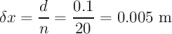 | (2.3) |
Therefore to achieve a Courant number less than or equal to 1 throughout the domain the time step deltaT must be set to less than or equal to:
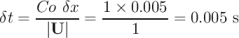 | (2.4) |
As the simulation progresses we wish to write results at certain intervals of time
that we can later view with a post-processing package. The writeControl
keyword presents several options for setting the time at which the results are
written; here we select the timeStep option which specifies that results are
written every  th time step where the value is specified under the
writeInterval keyword. Let us decide that we wish to write our results at times
0.1, 0.2,…, 0.5 s. With a time step of 0.005 s, we therefore need to output
results at every 20th time time step and so we set writeInterval to
20.
th time step where the value is specified under the
writeInterval keyword. Let us decide that we wish to write our results at times
0.1, 0.2,…, 0.5 s. With a time step of 0.005 s, we therefore need to output
results at every 20th time time step and so we set writeInterval to
20.
OpenFOAM creates a new directory named after the current time, e.g. 0.1 s, on each occasion that it writes a set of data, as discussed in full in User Guide section ??. In the icoFoam solver, it writes out the results for each field, U and p, into the time directories. For this case, the entries in the controlDict are shown below:
17
18application icoFoam;
19
20startFrom startTime;
21
22startTime 0;
23
24stopAt endTime;
25
26endTime 0.5;
27
28deltaT 0.005;
29
30writeControl timeStep;
31
32writeInterval 20;
33
34purgeWrite 0;
35
36writeFormat ascii;
37
38writePrecision 6;
39
40writeCompression off;
41
42timeFormat general;
43
44timePrecision 6;
45
46runTimeModifiable true;
47
48
49// ************************************************************************* //
2.1.1.5 Discretisation and linear-solver settings
The user specifies the choice of finite volume discretisation schemes in the fvSchemes dictionary in the system directory. The specification of the linear equation solvers and tolerances and other algorithm controls is made in the fvSolution dictionary, similarly in the system directory. The user is free to view these dictionaries but we do not need to discuss all their entries at this stage except for pRefCell and pRefValue in the PISO sub-dictionary of the fvSolution dictionary. In a closed incompressible system such as the cavity, pressure is relative: it is the pressure range that matters not the absolute values. In cases such as this, the solver sets a reference level by pRefValue in cell pRefCell. In this example both are set to 0. Changing either of these values will change the absolute pressure field, but not, of course, the relative pressures or velocity field.
2.1.2 Viewing the mesh
Before the case is run it is a good idea to view the mesh to check for any errors. The mesh is viewed in paraFoam, the post-processing tool supplied with OpenFOAM. The paraFoam post-processing is started by typing in the terminal from within the case directory
paraFoam
Alternatively, it can be launched from another directory location with an optional -case argument giving the case directory, e.g.
paraFoam -case $FOAM_RUN/tutorials/incompressible/icoFoam/cavity/cavity
This launches the ParaView window as shown in Figure ??. In the Pipeline Browser, the user can see that ParaView has opened cavity.OpenFOAM, the module for the cavity case. Before clicking the Apply button, the user needs to select some geometry from the Mesh Parts panel. Because the case is small, it is easiest to select all the data by checking the box adjacent to the Mesh Parts panel title, which automatically checks all individual components within the respective panel. The user should then click the Apply button to load the geometry into ParaView. Some general settings are applied as described in User Guide section ??. Please consult this section about these settings.
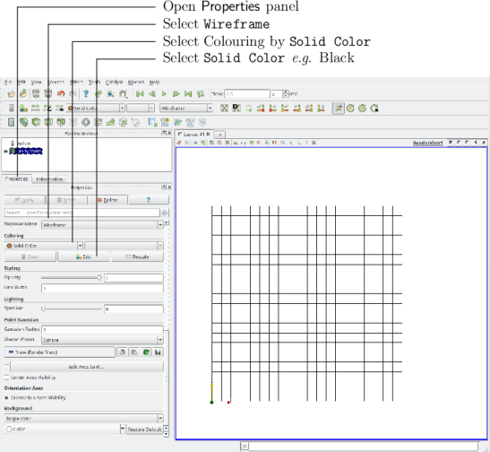
The user should then open the Properties panel that controls the visual representation of the selected module. Within the Display panel the user should do the following as shown in Figure 2.3: (1) set Color By Solid Color; (2) click Edit and select an appropriate colour e.g. black (for a white background); (3) select Wireframe from the Representation menu. The background colour can be set by selecting Settings… from Edit in the top menu panel.
Especially the first time the user starts ParaView, it is recommended that they manipulate the view as described in User Guide section ??. In particular, since this is a 2D case, it is recommended that Camera Parallel Projection is selected. To do so, click on the Toggle Advanced Properties to show the option towards the bottom on the panel. The Orientation Axes can be toggled on and off in the Annotation window or moved by drag and drop with the mouse.
2.1.3 Running an application
Like any UNIX/Linux executable, OpenFOAM applications can be run in two ways: as a foreground process, i.e. one in which the shell waits until the command has finished before giving a command prompt; as a background process, one which does not have to be completed before the shell accepts additional commands.
On this occasion, we will run icoFoam in the foreground. The icoFoam solver is executed either by entering the case directory and typing
icoFoam
icoFoam -case $FOAM_RUN/tutorials/incompressible/icoFoam/cavity/cavity
The progress of the job is written to the terminal window. It tells the user the current time, maximum Courant number, initial and final residuals for all fields.
2.1.4 Post-processing
As soon as results are written to time directories, they can be viewed using paraFoam. Return to the paraFoam window and select the Properties panel for the cavity.OpenFOAM case module. If the correct window panels for the case module do not seem to be present at any time, please ensure that: cavity.OpenFOAM is highlighted in blue; eye button alongside it is switched on to show the graphics are enabled;
To prepare paraFoam to display the data of interest, we must first load the data at the required run time of 0.5 s. If the case was run while ParaView was open, the output data in time directories will not be automatically loaded within ParaView. To load the data the user should click Refresh Times in the Properties window. The time data will be loaded into ParaView.
2.1.4.1 Isosurface and contour plots
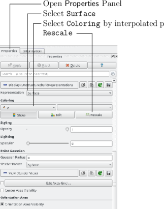
To view pressure, the user should open the Properties panel since it controls the
visual representation of the selected module. To make a simple plot of pressure,
the user should select the following, as described in detail in Figure 2.4: select
Surface from the Representation menu; in the Coloring panel, select Color by
![]() and Rescale to Data Range. Now in order to view the solution at
and Rescale to Data Range. Now in order to view the solution at
 s, the user can use the VCR Controls or Current Time Controls to
change the current time to 0.5. These are located in the toolbars below the menus
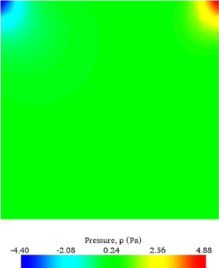
at the top of the ParaView window, as shown in Figure ??. The pressure field
solution has, as expected, a region of low pressure at the top left of the
cavity and one of high pressure at the top right of the cavity as shown in
Figure 2.5.
s, the user can use the VCR Controls or Current Time Controls to
change the current time to 0.5. These are located in the toolbars below the menus
at the top of the ParaView window, as shown in Figure ??. The pressure field
solution has, as expected, a region of low pressure at the top left of the
cavity and one of high pressure at the top right of the cavity as shown in
Figure 2.5.
With the point icon (![]() ) the pressure field is interpolated across each cell
to give a continuous appearance. Instead if the user selects the cell icon,
) the pressure field is interpolated across each cell
to give a continuous appearance. Instead if the user selects the cell icon, ![]() ,
from the Coloring by menu, a single value for pressure will be attributed
to each cell so that each cell will be denoted by a single colour with no
grading.
,
from the Coloring by menu, a single value for pressure will be attributed
to each cell so that each cell will be denoted by a single colour with no
grading.
A colour bar can be included by either by clicking the Toggle Color Legend Visibility button in the Active Variable Controls toolbar, or by selecting Show Color Legend from the View menu. Clicking the Edit Color Map button, either in the Active Variable Controls toolbar or in the Color panel of the Display window, the user can set a range of attributes of the colour bar, such as text size, font selection and numbering format for the scale. The colour bar can be located in the image window by drag and drop with the mouse.
New versions of ParaView default to using a colour scale of blue to white to red rather than the more common blue to green to red (rainbow). Therefore the first time that the user executes ParaView, they may wish to change the colour scale. This can be done by selecting Choose Preset in the Color Scale Editor and selecting Blue to Red Rainbow. After clicking the OK confirmation button, the user can click the Make Default button so that ParaView will always adopt this type of colour bar.
If the user rotates the image, they can see that they have now coloured the
complete geometry surface by the pressure. In order to produce a genuine contour
plot the user should first create a cutting plane, or ‘slice’, through the geometry
using the Slice filter as described in User Guide section ??. The cutting plane
should be centred at 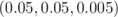 and its normal should be set to
  (click the Z Normal button). Having generated the cutting plane, the
contours can be created using by the Contour filter described in User
Guide section ??.
(click the Z Normal button). Having generated the cutting plane, the
contours can be created using by the Contour filter described in User
Guide section ??.
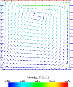
2.1.4.2 Vector plots
Before we start to plot the vectors of the flow velocity, it may be useful to remove other modules that have been created, e.g. using the Slice and Contour filters described above. These can: either be deleted entirely, by highlighting the relevant module in the Pipeline Browser and clicking Delete in their respective Properties panel; or, be disabled by toggling the eye button for the relevant module in the Pipeline Browser.
We now wish to generate a vector glyph for velocity at the centre of each cell. We first need to filter the data to cell centres as described in User Guide section ??. With the cavity.OpenFOAM module highlighted in the Pipeline Browser, the user should select Cell Centers from the Filter->Alphabetical menu and then click Apply.
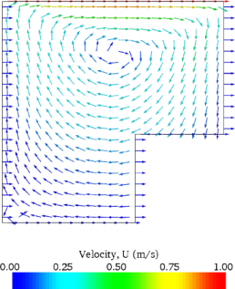
With these Centers highlighted in the Pipeline Browser, the user should then select Glyph from the Filter->Alphabetical menu. The Properties window panel should appear as shown in Figure 2.6. In the resulting Properties panel, the velocity field, U, is automatically selected in the vectors menu, since it is the only vector field present. By default the Scale Mode for the glyphs will be Vector Magnitude of velocity but, since the we may wish to view the velocities throughout the domain, the user should instead select off and Set Scale Factor to 0.005. On clicking Apply, the glyphs appear coloured by pressure. The user should also select Show Color Legend in Edit Color Map. The output is shown in Figure 2.7, in which uppercase Times Roman fonts are selected for the Color Legend headings and the labels are specified to 2 fixed significant figures by deselecting Automatic Label Format and entering %-#6.2f in the Label Format text box. The background colour is set to white in the Properties as described in User Guide section ??.
Note that at the left and right walls, glyphs appear to indicate flow through
the walls. On closer examination, however, the user can see that while the flow
direction is normal to the wall, its magnitude is 0. This slightly confusing
situation is caused by ParaView choosing to orientate the glyphs in the
 -direction when the glyph scaling off and the velocity magnitude is
0.
-direction when the glyph scaling off and the velocity magnitude is
0.
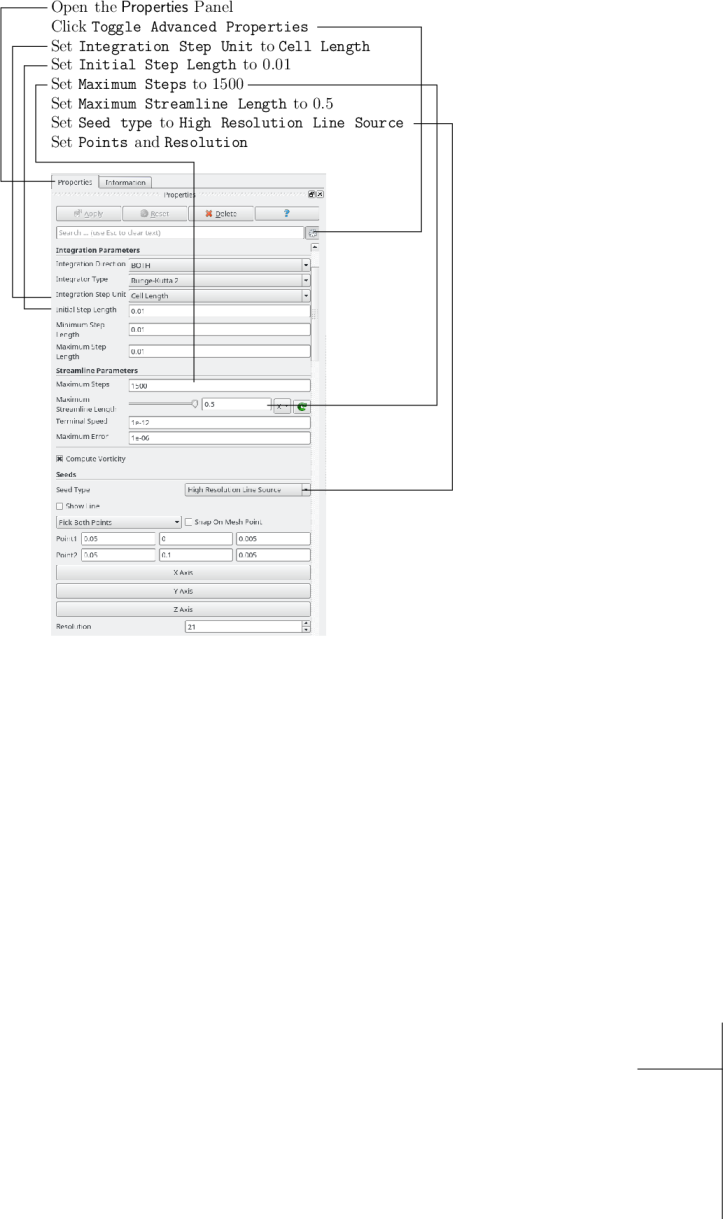
2.1.4.3 Streamline plots
Again, before the user continues to post-process in ParaView, they should disable modules such as those for the vector plot described above. We now wish to plot streamlines of velocity as described in User Guide section ??.
With the cavity.OpenFOAM module highlighted in the Pipeline Browser, the
user should then select Stream Tracer from the Filter menu and then click
Apply. The Properties window panel should appear as shown in Figure 2.8. The
Seed points should be specified along a Line Source running vertically through
the centre of the geometry, i.e. from  to
to  . For the
image in this guide we used: a point Resolution of 21; Max Propagation by
Length 0.5; Initial Step Length by Cell Length 0.01; and, Integration
Direction BOTH. The Runge-Kutta 2 IntegratorType was used with default
parameters.
. For the
image in this guide we used: a point Resolution of 21; Max Propagation by
Length 0.5; Initial Step Length by Cell Length 0.01; and, Integration
Direction BOTH. The Runge-Kutta 2 IntegratorType was used with default
parameters.
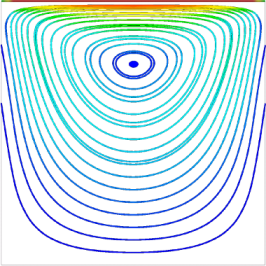
On clicking Apply the tracer is generated. The user should then select Tube from the Filter menu to produce high quality streamline images. For the image in this report, we used: Num. sides 6; Radius 0.0003; and, Radius factor 10. The streamtubes are coloured by velocity magnitude. On clicking Apply the image in Figure 2.9 should be produced.
2.1.5 Increasing the mesh resolution
The mesh resolution will now be increased by a factor of two in each direction. The results from the coarser mesh will be mapped onto the finer mesh to use as initial conditions for the problem. The solution from the finer mesh will then be compared with those from the coarser mesh.
2.1.5.1 Creating a new case using an existing case
We now wish to create a new case named cavityFine that is created from cavity. The user should therefore clone the cavity case and edit the necessary files. First the user should create a new case directory at the same directory level as the cavity case, e.g.
cd $FOAM_RUN/tutorials/incompressible/icoFoam/cavity
mkdir cavityFine
cp -r cavity/constant cavityFine
cp -r cavity/system cavityFine
cd cavityFine
2.1.5.2 Creating the finer mesh
We now wish to increase the number of cells in the mesh by using blockMesh. The user should open the blockMeshDict file in an editor and edit the block specification. The blocks are specified in a list under the blocks keyword. The syntax of the block definitions is described fully in User Guide section ??; at this stage it is sufficient to know that following hex is first the list of vertices in the block, then a list (or vector) of numbers of cells in each direction. This was originally set to (20 20 1) for the cavity case. The user should now change this to (40 40 1) and save the file. The new refined mesh should then be created by running blockMesh as before.
2.1.5.3 Mapping the coarse mesh results onto the fine mesh
The mapFields utility maps one or more fields relating to a given geometry onto the corresponding fields for another geometry. In our example, the fields are deemed ‘consistent’ because the geometry and the boundary types, or conditions, of both source and target fields are identical. We use the -consistent command line option when executing mapFields in this example.
The field data that mapFields maps is read from the time directory specified by startFrom/startTime in the controlDict of the target case, i.e. those into which the results are being mapped. In this example, we wish to map the final results of the coarser mesh from case cavity onto the finer mesh of case cavityFine. Therefore, since these results are stored in the 0.5 directory of cavity, the startTime should be set to 0.5 s in the controlDict dictionary and startFrom should be set to startTime.
The case is ready to run mapFields. Typing mapFields -help quickly shows that mapFields requires the source case directory as an argument. We are using the -consistent option, so the utility is executed from within the cavityFine directory by
mapFields ../cavity -consistent
Source: ".." "cavity"
Target: "." "cavityFine"
Create databases as time
Source time: 0.5
Target time: 0.5
Create meshes
Source mesh size: 400 Target mesh size: 1600
Consistently creating and mapping fields for time 0.5
interpolating p
interpolating U
End
Target: "." "cavityFine"
Create databases as time
Source time: 0.5
Target time: 0.5
Create meshes
Source mesh size: 400 Target mesh size: 1600
Consistently creating and mapping fields for time 0.5
interpolating p
interpolating U
End
2.1.5.4 Control adjustments
To maintain a Courant number of less that 1, as discussed in section 2.1.1.4, the time step must now be halved since the size of all cells has halved. Therefore deltaT should be set to to 0.0025 s in the controlDict dictionary. Field data is currently written out at an interval of a fixed number of time steps. Here we demonstrate how to specify data output at fixed intervals of time. Under the writeControl keyword in controlDict, instead of requesting output by a fixed number of time steps with the timeStep entry, a fixed amount of run time can be specified between the writing of results using the runTime entry. In this case the user should specify output every 0.1 and therefore should set writeInterval to 0.1 and writeControl to runTime. Finally, since the case is starting with a the solution obtained on the coarse mesh we only need to run it for a short period to achieve reasonable convergence to steady-state. Therefore the endTime should be set to 0.7 s. Make sure these settings are correct and then save the file.
2.1.5.5 Running the code as a background process
The user should experience running icoFoam as a background process, redirecting the terminal output to a log file that can be viewed later. From the cavityFine directory, the user should execute:
icoFoam > log &
cat log
2.1.5.6 Vector plot with the refined mesh
The user can open multiple cases simultaneously in ParaView; essentially because each new case is simply another module that appears in the Pipeline Browser. There is one minor inconvenience when opening a new case in ParaView because there is a prerequisite that the selected data is a file with a name that has an extension. However, in OpenFOAM, each case is stored in a multitude of files with no extensions within a specific directory structure. The solution, that the paraFoam script performs automatically, is to create a dummy file with the extension .OpenFOAM — hence, the cavity case module is called cavity.OpenFOAM.
However, if the user wishes to open another case directly from within ParaView, they need to create such a dummy file. For example, to load the cavityFine case the file would be created by typing at the command prompt:
cd $FOAM_RUN/tutorials/incompressible/icoFoam/cavity
touch cavityFine/cavityFine.OpenFOAM
Now the cavityFine case can be loaded into ParaView by selecting Open from the File menu, and having navigated the directory tree, selecting cavityFine.OpenFOAM. The user can now make a vector plot of the results from the refined mesh in ParaView. The plot can be compared with the cavity case by enabling glyph images for both case simultaneously.
2.1.5.7 Plotting graphs
The user may wish to visualise the results by extracting some scalar measure of velocity and plotting 2-dimensional graphs along lines through the domain. OpenFOAM is well equipped for this kind of data manipulation. There are numerous utilities that perform specialised data manipulations, and many can be accessed via the postProcess utility:
postProcess -list
CourantNo
Lambda2
MachNo
PecletNo
Q
R
XiReactionRate
add
boundaryCloud
cellMax
cellMin
components
div
enstrophy
faceMax
faceMin
flowRatePatch
flowType
forceCoeffsCompressible
forceCoeffsIncompressible
forcesCompressible
forcesIncompressible
grad
internalCloud
mag
magSqr
minMaxComponents
minMaxMagnitude
patchAverage
patchIntegrate
pressureDifferencePatch
pressureDifferenceSurface
probes
randomise
residuals
scalarTransport
singleGraph
staticPressure
streamFunction
streamlines
subtract
surfaces
totalPressureCompressible
totalPressureIncompressible
turbulenceFields
volFlowRateSurface
vorticity
wallHeatFlux
wallShearStress
writeCellCentres
writeCellVolumes
writeObjects
yPlus
When the components function is run on a case, say cavity, it reads the
velocity vector field from each time directory and, in the corresponding
time directories, writes scalar fields Ux, Uy and Uz representing the  ,
,
 and
and  components of velocity. Similarly the mag function writes a
scalar field magU to each time directory representing the magnitude of
velocity.
components of velocity. Similarly the mag function writes a
scalar field magU to each time directory representing the magnitude of
velocity.
The user can run both functions simultaneously, e.g. for the cavity case the user should go into the cavity directory and execute postProcess as follows:
cd $FOAM RUN/tutorials/incompressible/icoFoam/cavity/cavity
postProcess -funcs '(components(U) mag(U))'
The individual components can be plotted as a graph in ParaView. It is quick, convenient and has reasonably good control over labelling and formatting, so the printed output is a fairly good standard. However, to produce graphs for publication, users may prefer to write raw data and plot it with a dedicated graphing tool, such as gnuplot or Grace/xmgr. To do this, see section 5.1.4.
Before commencing plotting, the user needs to load the newly generated Ux, Uy and Uz fields into ParaView. To do this, the user should click the Refresh button at the top of the Properties panel for the cavity.OpenFOAM module which will cause the new fields to be loaded into ParaView and appear in the Volume Fields window. Ensure the new fields are selected and the changes are applied, i.e. click Apply again if necessary. Also, data is interpolated incorrectly at boundaries if the boundary regions are selected in the Mesh Parts panel. Therefore the user should deselect the patches in the Mesh Parts panel, i.e.movingWall, fixedWall and frontAndBack, and apply the changes.
Now, in order to display a graph in ParaView the user should select the
module of interest, e.g.cavity.OpenFOAM and apply the Plot Over Line filter
from the Filter->Data Analysis menu. This opens up a new XY Plot
window below or beside the existing 3D View window. A PlotOverLine
module is created in which the user can specify the end points of the
line in the Properties panel. In this example, the user should position the
line vertically up the centre of the domain, i.e. from  to
to
 , in the Point1 and Point2 text boxes. The Resolution can be set
to 100.
, in the Point1 and Point2 text boxes. The Resolution can be set
to 100.
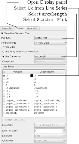
On clicking Apply, a graph is generated in the XY Plot window. In the Display panel, the Attribute Mode is set to Point Data by default. The Use Data Array option can be selected for the X Axis Data, taking the arc_length option so that the x-axis of the graph represents distance from the base of the cavity.
The user can choose the fields to be displayed in the Line Series panel of the Display window. From the list of scalar fields to be displayed, it can be seen that the magnitude and components of vector fields are available by default, e.g. displayed as U:X, so that it was not necessary to create Ux using postProcess. Nevertheless, the user should deselect all series except Ux (or U:x). A square colour box in the adjacent column to the selected series indicates the line colour. The user can edit this most easily by a double click of the mouse over that selection.
In order to format the graph, the user should modify the settings below the Line Series panel, namely Line Color, Line Thickness, Line Style, Marker Style and Chart Axes.
Also the user can click one of the buttons above the top left corner of the XY Plot. The third button, for example, allows the user to control View Settings in which the user can set title and legend for each axis, for example. Also, the user can set font, colour and alignment of the axes titles, and has several options for axis range and labels in linear or logarithmic scales.
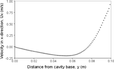
Figure 2.11 is a graph produced using ParaView. The user can produce a graph however he/she wishes. For information, the graph in Figure 2.11 was produced with the options for axes of: Standard type of Notation; Specify Axis Range selected; titles in Sans Serif 12 font. The graph is displayed as a set of points rather than a line by activating the Enable Line Series button in the Display window. Note: if this button appears to be inactive by being “greyed out”, it can be made active by selecting and deselecting the sets of variables in the Line Series panel. Once the Enable Line Series button is selected, the Line Style and Marker Style can be adjusted to the user’s preference.
2.1.6 Introducing mesh grading
The error in any solution will be more pronounced in regions where the form of the true solution differ widely from the form assumed in the chosen numerical schemes. For example a numerical scheme based on linear variations of variables over cells can only generate an exact solution if the true solution is itself linear in form. The error is largest in regions where the true solution deviates greatest from linear form, i.e. where the change in gradient is largest. Error decreases with cell size.
It is useful to have an intuitive appreciation of the form of the solution before setting up any problem. It is then possible to anticipate where the errors will be largest and to grade the mesh so that the smallest cells are in these regions. In the cavity case the large variations in velocity can be expected near a wall and so in this part of the tutorial the mesh will be graded to be smaller in this region. By using the same number of cells, greater accuracy can be achieved without a significant increase in computational cost.
A mesh of  cells with grading towards the walls will be created for the
lid-driven cavity problem and the results from the finer mesh of section 2.1.5.2
will then be mapped onto the graded mesh to use as an initial condition.
The results from the graded mesh will be compared with those from the
previous meshes. Since the changes to the blockMeshDict dictionary are
fairly substantial, the case used for this part of the tutorial, cavityGrade,
is supplied in the $FOAM_RUN/tutorials/incompressible/icoFoam/cavity
directory.
cells with grading towards the walls will be created for the
lid-driven cavity problem and the results from the finer mesh of section 2.1.5.2
will then be mapped onto the graded mesh to use as an initial condition.
The results from the graded mesh will be compared with those from the
previous meshes. Since the changes to the blockMeshDict dictionary are
fairly substantial, the case used for this part of the tutorial, cavityGrade,
is supplied in the $FOAM_RUN/tutorials/incompressible/icoFoam/cavity
directory.
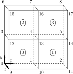
2.1.6.1 Creating the graded mesh
The mesh now needs 4 blocks as different mesh grading is needed on the left and right and top and bottom of the domain. The block structure for this mesh is shown in Figure 2.12.
The user can view the blockMeshDict file in the system subdirectory of
cavityGrade; for completeness the key elements of the blockMeshDict file are also
reproduced below. Each block now has  cells in the
  and
and  directions and
the ratio between largest and smallest cells is
directions and
the ratio between largest and smallest cells is  .
.
17scale 0.1;
18
19vertices
20(
21 (0 0 0)
22 (0.5 0 0)
23 (1 0 0)
24 (0 0.5 0)
25 (0.5 0.5 0)
26 (1 0.5 0)
27 (0 1 0)
28 (0.5 1 0)
29 (1 1 0)
30 (0 0 0.1)
31 (0.5 0 0.1)
32 (1 0 0.1)
33 (0 0.5 0.1)
34 (0.5 0.5 0.1)
35 (1 0.5 0.1)
36 (0 1 0.1)
37 (0.5 1 0.1)
38 (1 1 0.1)
39);
40
41blocks
42(
43 hex (0 1 4 3 9 10 13 12) (10 10 1) simpleGrading (2 2 1)
44 hex (1 2 5 4 10 11 14 13) (10 10 1) simpleGrading (0.5 2 1)
45 hex (3 4 7 6 12 13 16 15) (10 10 1) simpleGrading (2 0.5 1)
46 hex (4 5 8 7 13 14 17 16) (10 10 1) simpleGrading (0.5 0.5 1)
47);
48
49edges
50(
51);
52
53boundary
54(
55 movingWall
56 {
57 type wall;
58 faces
59 (
60 (6 15 16 7)
61 (7 16 17 8)
62 );
63 }
64 fixedWalls
65 {
66 type wall;
67 faces
68 (
69 (3 12 15 6)
70 (0 9 12 3)
71 (0 1 10 9)
72 (1 2 11 10)
73 (2 5 14 11)
74 (5 8 17 14)
75 );
76 }
77 frontAndBack
78 {
79 type empty;
80 faces
81 (
82 (0 3 4 1)
83 (1 4 5 2)
84 (3 6 7 4)
85 (4 7 8 5)
86 (9 10 13 12)
87 (10 11 14 13)
88 (12 13 16 15)
89 (13 14 17 16)
90 );
91 }
92);
93
94mergePatchPairs
95(
96);
97
98// ************************************************************************* //
Once familiar with the blockMeshDict file for this case, the user can execute blockMesh from the command line. The graded mesh can be viewed as before using paraFoam as described in section 2.1.2.
2.1.6.2 Changing time and time step
The highest velocities and smallest cells are next to the lid, therefore the highest Courant number will be generated next to the lid, for reasons given in section 2.1.1.4. It is therefore useful to estimate the size of the cells next to the lid to calculate an appropriate time step for this case.
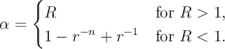
When a nonuniform mesh grading is used, blockMesh calculates the cell sizes
using a geometric progression. Along a length  , if
, if  cells are requested with a
ratio of
cells are requested with a
ratio of  between the last and first cells, the size of the smallest cell,
  , is
given by:
, is
given by:
 | (2.5) |
where  is the ratio between one cell size and the next which is given
by:
is the ratio between one cell size and the next which is given
by:
 | (2.6) |
and
 | (2.7) |
For the cavityGrade case the number of cells in each direction in a block
is 10, the ratio between largest and smallest cells is  and the block
height and width is 0.05
and the block
height and width is 0.05  . Therefore the smallest cell length is 3.45
 . From Equation 2.2, the time step should be less than 3.45
  to
maintain a Courant of less than 1. To ensure that results are written out at
convenient time intervals, the time step deltaT should be reduced to 2.5
to
maintain a Courant of less than 1. To ensure that results are written out at
convenient time intervals, the time step deltaT should be reduced to 2.5
 and the writeInterval set to 40 so that results are written out every
0.1 s. These settings can be viewed in the cavityGrade/system/controlDict
file.
and the writeInterval set to 40 so that results are written out every
0.1 s. These settings can be viewed in the cavityGrade/system/controlDict
file.
The startTime needs to be set to that of the final conditions of the case cavityFine, i.e.0.7. Since cavity and cavityFine converged well within the prescribed run time, we can set the run time for case cavityGrade to 0.1 s, i.e. the endTime should be 0.8.
2.1.6.3 Mapping fields
As in section 2.1.5.3, use mapFields to map the final results from case cavityFine onto the mesh for case cavityGrade. Enter the cavityGrade directory and execute mapFields by:
cd $FOAM_RUN/tutorials/incompressible/icoFoam/cavity/cavityGrade
mapFields ../cavityFine -consistent
Now run icoFoam from the case directory and monitor the run time information. View the converged results for this case and compare with other results using post-processing tools described previously in section 2.1.5.6 and section 2.1.5.7.
2.1.7 Increasing the Reynolds number
The cases solved so far have had a Reynolds number of 10. This is very low and leads to a stable solution quickly with only small secondary vortices at the bottom corners of the cavity. We will now increase the Reynolds number to 100, at which point the solution takes a noticeably longer time to converge. The coarsest mesh in case cavity will be used initially. The user should make a copy of the cavity case and name it cavityHighRe by typing:
cd $FOAM_RUN/tutorials/incompressible/icoFoam/cavity
cp -r cavity cavityHighRe
2.1.7.1 Pre-processing
Enter the cavityHighRe case and edit the transportProperties dictionary. Since the
Reynolds number is required to be increased by a factor of 10, decrease the
kinematic viscosity by a factor of 10, i.e. to 
 . We can now run
this case by restarting from the solution at the end of the cavity case run. To do
this we can use the option of setting the startFrom keyword to latestTime so
that icoFoam takes as its initial data the values stored in the directory
corresponding to the most recent time, i.e. 0.5. The endTime should be set to
2 s.
. We can now run
this case by restarting from the solution at the end of the cavity case run. To do
this we can use the option of setting the startFrom keyword to latestTime so
that icoFoam takes as its initial data the values stored in the directory
corresponding to the most recent time, i.e. 0.5. The endTime should be set to
2 s.
2.1.7.2 Running the code
Run icoFoam for this case from the case directory and view the run time information. When running a job in the background, the following UNIX commands can be useful:
- nohup
- enables a command to keep running after the user who issues the command has logged out;
- nice
- changes the priority of the job in the kernel’s scheduler; a niceness of -20 is the highest priority and 19 is the lowest priority.
This is useful, for example, if a user wishes to set a case running on a remote machine and does not wish to monitor it heavily, in which case they may wish to give it low priority on the machine. In that case the nohup command allows the user to log out of a remote machine he/she is running on and the job continues running, while nice can set the priority to 19. For our case of interest, we can execute the command in this manner as follows:
cd $FOAM_RUN/tutorials/incompressible/icoFoam/cavity/cavityHighRe
nohup nice -n 19 icoFoam > log &
cat log
 ), the
run has effectively converged and can be stopped once the field data has been
written out to a time directory. For example, at convergence a sample of
the log file from the run on the cavityHighRe case appears as follows in
which the velocity has already converged after 1.62 s and initial pressure
residuals are small; No Iterations 0 indicates that the solution of U has
stopped:
), the
run has effectively converged and can be stopped once the field data has been
written out to a time directory. For example, at convergence a sample of
the log file from the run on the cavityHighRe case appears as follows in
which the velocity has already converged after 1.62 s and initial pressure
residuals are small; No Iterations 0 indicates that the solution of U has
stopped:
1
2Time = 1.63
3
4Courant Number mean: 0.221985 max: 0.839923
5smoothSolver: Solving for Ux, Initial residual = 3.64032e-06, Final residual = 3.64032e-06, No Iterations 0
6smoothSolver: Solving for Uy, Initial residual = 4.20677e-06, Final residual = 4.20677e-06, No Iterations 0
7DICPCG: Solving for p, Initial residual = 2.11678e-06, Final residual = 7.25303e-07, No Iterations 3
8time step continuity errors : sum local = 7.25166e-09, global = 4.96308e-19, cumulative = -1.28342e-17
9DICPCG: Solving for p, Initial residual = 1.36075e-06, Final residual = 7.94478e-07, No Iterations 1
10time step continuity errors : sum local = 7.77548e-09, global = -4.78772e-19, cumulative = -1.3313e-17
11ExecutionTime = 0.38 s ClockTime = 0 s
12
13Time = 1.635
14
15Courant Number mean: 0.221986 max: 0.839923
16smoothSolver: Solving for Ux, Initial residual = 3.56036e-06, Final residual = 3.56036e-06, No Iterations 0
17smoothSolver: Solving for Uy, Initial residual = 4.11726e-06, Final residual = 4.11726e-06, No Iterations 0
18DICPCG: Solving for p, Initial residual = 2.03881e-06, Final residual = 8.18692e-07, No Iterations 3
19time step continuity errors : sum local = 8.38471e-09, global = -6.27334e-19, cumulative = -1.39403e-17
20DICPCG: Solving for p, Initial residual = 1.36655e-06, Final residual = 7.94623e-07, No Iterations 1
21time step continuity errors : sum local = 8.25673e-09, global = 5.87298e-20, cumulative = -1.38816e-17
22ExecutionTime = 0.38 s ClockTime = 0 s
2.1.8 High Reynolds number flow
View the results in paraFoam and display the velocity vectors. The secondary vortices in the corners have increased in size somewhat. The user can then increase the Reynolds number further by decreasing the viscosity and then rerun the case. The number of vortices increases so the mesh resolution around them will need to increase in order to resolve the more complicated flow patterns. In addition, as the Reynolds number increases the time to convergence increases. The user should monitor residuals and extend the endTime accordingly to ensure convergence.
The need to increase spatial and temporal resolution then becomes impractical
as the flow moves into the turbulent regime, where problems of solution stability
may also occur. Of course, many engineering problems have very high Reynolds
numbers and it is infeasible to bear the huge cost of solving the turbulent
behaviour directly. Instead Reynolds-averaged simulation (RAS) turbulence
models are used to solve for the mean flow behaviour and calculate the statistics
of the fluctuations. The standard  model with wall functions will be used in
this tutorial to solve the lid-driven cavity case with a Reynolds number of
model with wall functions will be used in
this tutorial to solve the lid-driven cavity case with a Reynolds number of
 . Two extra variables are solved for:
  , the turbulent kinetic energy;
and,
, the turbulent kinetic energy;
and,  , the turbulent dissipation rate. The additional equations and
models for turbulent flow are implemented into a OpenFOAM solver called
pisoFoam.
, the turbulent dissipation rate. The additional equations and
models for turbulent flow are implemented into a OpenFOAM solver called
pisoFoam.
2.1.8.1 Pre-processing
Change directory to the cavity case in the $FOAM_RUN/tutorials/incompressible/pisoFoam/RAS
directory (N.B: the pisoFoam/RAS directory). Generate the mesh by running
blockMesh as before. Mesh grading towards the wall is not necessary when using
the standard  model with wall functions since the flow in the near wall cell
is modelled, rather than having to be resolved.
model with wall functions since the flow in the near wall cell
is modelled, rather than having to be resolved.
A range of wall function models is available in OpenFOAM that are applied as
boundary conditions on individual patches. This enables different wall function
models to be applied to different wall regions. The choice of wall function
models are specified through the turbulent viscosity field,  in the 0/nut
file:
in the 0/nut
file:
17
18dimensions [0 2 -1 0 0 0 0];
19
20internalField uniform 0;
21
22boundaryField
23{
24 movingWall
25 {
26 type nutkWallFunction;
27 value uniform 0;
28 }
29 fixedWalls
30 {
31 type nutkWallFunction;
32 value uniform 0;
33 }
34 frontAndBack
35 {
36 type empty;
37 }
38}
39
40
41// ************************************************************************* //
This case uses standard wall functions, specified by the nutWallFunction keyword entry on the movingWall and fixedWalls patches. Other wall function models include the rough wall functions, specified though the nutRoughWallFunction keyword.
The user should now open the field files for  and
and  (0/k and 0/epsilon) and
examine their boundary conditions. For a wall boundary condition wall, is
assigned a epsilonWallFunction boundary condition and a kqRwallFunction
boundary condition is assigned to
(0/k and 0/epsilon) and
examine their boundary conditions. For a wall boundary condition wall, is
assigned a epsilonWallFunction boundary condition and a kqRwallFunction
boundary condition is assigned to  . The latter is a generic boundary condition
that can be applied to any field that are of a turbulent kinetic energy type,
e.g.
. The latter is a generic boundary condition
that can be applied to any field that are of a turbulent kinetic energy type,
e.g.  ,
,  or Reynolds Stress
  . The initial values for
  and
and  are set
using an estimated fluctuating component of velocity
are set
using an estimated fluctuating component of velocity  and a turbulent
length scale,
and a turbulent
length scale,  .
.  and
and  are defined in terms of these parameters as
follows:
are defined in terms of these parameters as
follows:
where  is a constant of the
  model equal to 0.09. For a Cartesian
coordinate system,
model equal to 0.09. For a Cartesian
coordinate system,  is given by:
 | (2.10) |
where  ,
,  and
and  are the fluctuating components of velocity in the
 ,
,  and
and  directions respectively. Let us assume the initial turbulence is
isotropic, i.e.
directions respectively. Let us assume the initial turbulence is
isotropic, i.e.  , and equal to 5% of the lid velocity and that
  ,
is equal to 20% of the box width, 0.1
,
is equal to 20% of the box width, 0.1  , then
  and
and  are given
by:
are given
by:

These form the initial conditions for  and
and  . The initial conditions for
  and
and  are
are  and 0 respectively as before.
Turbulence modelling includes a range of methods, e.g. RAS or large-eddy simulation (LES), that are provided in OpenFOAM. In most transient solvers, the choice of turbulence modelling method is selectable at run-time through the simulationType keyword in turbulenceProperties dictionary. The user can view this file in the constant directory:
17
18simulationType RAS;
19
20RAS
21{
22 RASModel kEpsilon;
23
24 turbulence on;
25
26 printCoeffs on;
27}
28
29// ************************************************************************* //
18simulationType RAS;
19
20RAS
21{
22 RASModel kEpsilon;
23
24 turbulence on;
25
26 printCoeffs on;
27}
28
29// ************************************************************************* //
The options for simulationType are laminar, RAS and LES. More informaton on
turbulence models can be found in the Extended Code Guide With RAS selected in
this case, the choice of RAS modelling is specified in a turbulenceProperties
subdictionary, also in the constant directory. The turbulence model is selected by
the RASModel entry from a long list of available models that are listed in User
Guide Table ??. The kEpsilon model should be selected which is is the standard
 model; the user should also ensure that turbulence calculation is switched
on.
model; the user should also ensure that turbulence calculation is switched
on.
The coefficients for each turbulence model are stored within the respective code with a set of default values. Setting the optional switch called printCoeffs to on will make the default values be printed to standard output, i.e. the terminal, when the model is called at run time. The coefficients are printed out as a sub-dictionary whose name is that of the model name with the word Coeffs appended, e.g. kEpsilonCoeffs in the case of the kEpsilon model. The coefficients of the model, e.g. kEpsilon, can be modified by optionally including (copying and pasting) that sub-dictionary within the turbulenceProperties file and adjusting values accordingly.
The user should next set the laminar kinematic viscosity in the transportProperties
dictionary. To achieve a Reynolds number of  , a kinematic viscosity of

 is required based on the Reynolds number definition given in
Equation 2.1.
is required based on the Reynolds number definition given in
Equation 2.1.
Finally the user should set the startTime, stopTime, deltaT and the writeInterval in the controlDict. Set deltaT to 0.005 s to satisfy the Courant number restriction and the endTime to 10 s.
2.1.8.2 Running the code
Execute pisoFoam by entering the case directory and typing “pisoFoam” in a
terminal. In this case, where the viscosity is low, the boundary layer next to the
moving lid is very thin and the cells next to the lid are comparatively large so the
velocity at their centres are much less than the lid velocity. In fact, after  100
time steps it becomes apparent that the velocity in the cells adjacent to the lid
reaches an upper limit of around 0.2
100
time steps it becomes apparent that the velocity in the cells adjacent to the lid
reaches an upper limit of around 0.2  hence the maximum Courant number
does not rise much above 0.2. It is sensible to increase the solution time by
increasing the time step to a level where the Courant number is much closer to 1.
Therefore reset deltaT to 0.02 s and, on this occasion, set startFrom to
latestTime. This instructs pisoFoam to read the start data from the latest
time directory, i.e.10.0. The endTime should be set to 20 s since the run
converges a lot slower than the laminar case. Restart the run as before and
monitor the convergence of the solution. View the results at consecutive
time steps as the solution progresses to see if the solution converges to a
steady-state or perhaps reaches some periodically oscillating state. In the latter
case, convergence may never occur but this does not mean the results are
inaccurate.
hence the maximum Courant number
does not rise much above 0.2. It is sensible to increase the solution time by
increasing the time step to a level where the Courant number is much closer to 1.
Therefore reset deltaT to 0.02 s and, on this occasion, set startFrom to
latestTime. This instructs pisoFoam to read the start data from the latest
time directory, i.e.10.0. The endTime should be set to 20 s since the run
converges a lot slower than the laminar case. Restart the run as before and
monitor the convergence of the solution. View the results at consecutive
time steps as the solution progresses to see if the solution converges to a
steady-state or perhaps reaches some periodically oscillating state. In the latter
case, convergence may never occur but this does not mean the results are
inaccurate.
2.1.9 Changing the case geometry
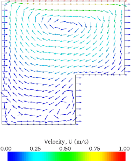
A user may wish to make changes to the geometry of a case and perform a new simulation. It may be useful to retain some or all of the original solution as the starting conditions for the new simulation. This is a little complex because the fields of the original solution are not consistent with the fields of the new case. However the mapFields utility can map fields that are inconsistent, either in terms of geometry or boundary types or both.
As an example, let us go to the cavityClipped case in the icoFoam directory
which consists of the standard cavity geometry but with a square of length
 removed from the bottom right of the cavity, according to the
blockMeshDict below:
removed from the bottom right of the cavity, according to the
blockMeshDict below:
17scale 0.1;
18
19vertices
20(
21 (0 0 0)
22 (0.6 0 0)
23 (0 0.4 0)
24 (0.6 0.4 0)
25 (1 0.4 0)
26 (0 1 0)
27 (0.6 1 0)
28 (1 1 0)
29
30 (0 0 0.1)
31 (0.6 0 0.1)
32 (0 0.4 0.1)
33 (0.6 0.4 0.1)
34 (1 0.4 0.1)
35 (0 1 0.1)
36 (0.6 1 0.1)
37 (1 1 0.1)
38
39);
40
41blocks
42(
43 hex (0 1 3 2 8 9 11 10) (12 8 1) simpleGrading (1 1 1)
44 hex (2 3 6 5 10 11 14 13) (12 12 1) simpleGrading (1 1 1)
45 hex (3 4 7 6 11 12 15 14) (8 12 1) simpleGrading (1 1 1)
46);
47
48edges
49(
50);
51
52boundary
53(
54 lid
55 {
56 type wall;
57 faces
58 (
59 (5 13 14 6)
60 (6 14 15 7)
61 );
62 }
63 fixedWalls
64 {
65 type wall;
66 faces
67 (
68 (0 8 10 2)
69 (2 10 13 5)
70 (7 15 12 4)
71 (4 12 11 3)
72 (3 11 9 1)
73 (1 9 8 0)
74 );
75 }
76 frontAndBack
77 {
78 type empty;
79 faces
80 (
81 (0 2 3 1)
82 (2 5 6 3)
83 (3 6 7 4)
84 (8 9 11 10)
85 (10 11 14 13)
86 (11 12 15 14)
87 );
88 }
89);
90
91mergePatchPairs
92(
93);
94
95// ************************************************************************* //
Generate the mesh with blockMesh. The patches are set as according to the previous cavity cases. For the sake of clarity in describing the field mapping process, the upper wall patch is renamed lid, previously the movingWall patch of the original cavity.
In an inconsistent mapping, there is no guarantee that all the field data can be mapped from the source case. The remaining data must come from field files in the target case itself. Therefore field data must exist in the time directory of the target case before mapping takes place. In the cavityClipped case the mapping is set to occur at time 0.5 s, since the startTime is set to 0.5 s in the controlDict. Therefore the user needs to copy initial field data to that directory, e.g. from time 0:
cd $FOAM_RUN/tutorials/incompressible/icoFoam/cavity/cavityClipped
cp -r 0 0.5
Now we wish to map the velocity and pressure fields from cavity onto the new fields of cavityClipped. Since the mapping is inconsistent, we need to edit the mapFieldsDict dictionary, located in the system directory. The dictionary contains 2 keyword entries: patchMap and cuttingPatches. The patchMap list contains a mapping of patches from the source fields to the target fields. It is used if the user wishes a patch in the target field to inherit values from a corresponding patch in the source field. In cavityClipped, we wish to inherit the boundary values on the lid patch from movingWall in cavity so we must set the patchMap as:
patchMap
(
lid movingWall
);
The cuttingPatches list contains names of target patches whose values are to be mapped from the source internal field through which the target patch cuts. In this case we will include the fixedWalls to demonstrate the interpolation process.
cuttingPatches
(
fixedWalls
);
Now the user should run mapFields, from within the cavityClipped directory:
mapFields ../cavity
 . Edit the U field, go to the fixedWalls patch and
change the field from nonuniform to uniform
. Edit the U field, go to the fixedWalls patch and
change the field from nonuniform to uniform  . The nonuniform field is a
list of values that requires deleting in its entirety. Now run the case with
icoFoam.
. The nonuniform field is a
list of values that requires deleting in its entirety. Now run the case with
icoFoam.
2.1.10 Post-processing the modified geometry
Velocity glyphs can be generated for the case as normal, first at time 0.5 s and later at time 0.6 s, to compare the initial and final solutions. In addition, we provide an outline of the geometry which requires some care to generate for a 2D case. The user should select Extract Block from the Filter menu and, in the Parameter panel, highlight the patches of interest, namely the lid and fixedWalls. On clicking Apply, these items of geometry can be displayed by selecting Wireframe in the Properties panel. Figure 2.14 displays the patches in black and shows vortices forming in the bottom corners of the modified geometry.