2.3 Magnetohydrodynamic flow of a liquid
Tutorial path:
In this example we shall investigate the flow of an electrically-conducting liquid through a magnetic field. The problem belongs to the branch of fluid dynamics known as magnetohydrodynamics (MHD), simulated using the mhdFoam solver.
2.3.1 Problem specification
This case is known as the Hartmann problem, chosen as it contains an analytical solution with which mhdFoam can be validated. It is defined as follows:
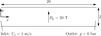
- Solution domain
- The domain is 2 dimensional and consists
of flow along two parallel plates as shown in Fig. 2.18.
- Governing equations
-
- Mass continuity for incompressible fluid

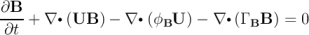
(2.16) - Momentum equation for incompressible fluid

(2.17) where
 is the magnetic flux density,
  .
.
- Maxwell’s equations
(2.18) where
 is the electric field strength.

(2.19) 
(2.20) assuming
 . Here,
  is the magnetic field strength,
  is
the current density and
is
the current density and  is the electric flux density.
- Charge continuity

(2.21) - Constitutive law

(2.22) - Ohm’s law
(2.23) - Combining Equation 2.18, Equation 2.20, Equation 2.23, and taking
the curl
(2.24)
- Mass continuity for incompressible fluid
- Boundary conditions
- Initial conditions
 ,
,  ,
,  .
.
- Transport properties
-
- Kinematic viscosity

- Density

- Electrical conductivity

- Permeability

- Kinematic viscosity
- Solver name
- mhdFoam: an incompressible laminar magneto-hydrodynamics code.
- Case name
- hartmann case located in the $FOAM_TUTORIALS/electromagnetics/mhdFoam directory.
 m/s;
m/s;
 ;
;
 .
.
2.3.2 Mesh generation
The geometry is simply modelled with 100 cells in the  -direction and 40 cells in
the
-direction and 40 cells in
the  -direction; the set of vertices and blocks are given in the mesh description
file below:
-direction; the set of vertices and blocks are given in the mesh description
file below:
1/*--------------------------------*- C++ -*----------------------------------*\
2| ========= | |
3| \\ / F ield | OpenFOAM: The Open Source CFD Toolbox |
4| \\ / O peration | Version: v2006 |
5| \\ / A nd | Website: www.openfoam.com |
6| \\/ M anipulation | |
7\*---------------------------------------------------------------------------*/
8FoamFile
9{
10 version 2.0;
11 format ascii;
12 class dictionary;
13 object blockMeshDict;
14}
15// * * * * * * * * * * * * * * * * * * * * * * * * * * * * * * * * * * * * * //
16
17scale 1;
18
19vertices
20(
21 (0 -1 0)
22 (20 -1 0)
23 (20 1 0)
24 (0 1 0)
25 (0 -1 0.1)
26 (20 -1 0.1)
27 (20 1 0.1)
28 (0 1 0.1)
29);
30
31blocks
32(
33 hex (0 1 2 3 4 5 6 7) (100 40 1) simpleGrading (1 1 1)
34);
35
36edges
37(
38);
39
40boundary
41(
42 inlet
43 {
44 type patch;
45 faces
46 (
47 (0 4 7 3)
48 );
49 }
50 outlet
51 {
52 type patch;
53 faces
54 (
55 (2 6 5 1)
56 );
57 }
58 lowerWall
59 {
60 type patch;
61 faces
62 (
63 (1 5 4 0)
64 );
65 }
66 upperWall
67 {
68 type patch;
69 faces
70 (
71 (3 7 6 2)
72 );
73 }
74 frontAndBack
75 {
76 type empty;
77 faces
78 (
79 (0 3 2 1)
80 (4 5 6 7)
81 );
82 }
83);
84
85mergePatchPairs
86(
87);
88
89// ************************************************************************* //
2.3.3 Running the case
The user can run the case and view results in ParaView. It is also useful at this
stage to run the Ucomponents utility to convert the  vector field into individual
scalar components. MHD flow is governed by, amongst other things, the
Hartmann number which is a measure of the ratio of electromagnetic body force
to viscous force
vector field into individual
scalar components. MHD flow is governed by, amongst other things, the
Hartmann number which is a measure of the ratio of electromagnetic body force
to viscous force
 | (2.25) |
where  is the characteristic length scale. In this case with
  ,
,
 and the electromagnetic body forces dominate the viscous forces.
Consequently with the flow fairly steady at
and the electromagnetic body forces dominate the viscous forces.
Consequently with the flow fairly steady at  the velocity profile
is almost planar, viewed at a cross section midway along the domain
the velocity profile
is almost planar, viewed at a cross section midway along the domain
 . The user can plot a graph of the profile of
  in dxFoam.
 and
and
 .
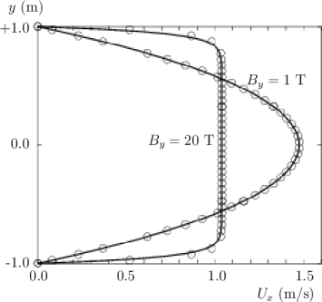
. Now the user should reduce the magnetic flux density  to 1
to 1  and re-run
the code and Ucomponents. In this case,
and re-run
the code and Ucomponents. In this case,  and the electromagnetic body
forces no longer dominate. The velocity profile consequently takes on the
parabolic form, characteristic of Poiseuille flow as shown in Figure 2.19. To
validate the code the analytical solution for the velocity profile
and the electromagnetic body
forces no longer dominate. The velocity profile consequently takes on the
parabolic form, characteristic of Poiseuille flow as shown in Figure 2.19. To
validate the code the analytical solution for the velocity profile  is
superimposed in Figure 2.19, given by:
is
superimposed in Figure 2.19, given by:
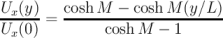 | (2.26) |
where the characteristic length  is half the width of the domain, i.e.
 .
.