OpenFOAM® v3.0+: New Post-processing Functionality

Image Creation during run time

The new runTimePostProcessing function object enables users to generate images both during, and after simulations. The object employs the VTK libraries to provide a broad set of functionality for scene composition and manipulation. Images are generated using a combination of function object output, and additional data e.g. triangulated surfaces and text. Current capabilities include support for:

• Camera
• Points
• Lines
• Surfaces
• Scalar bars
• Annotations
• Selection of colour maps

Scene configuration is performed using standard OpenFOAM dictionaries, using the main headings of: output, camera, colours, points, lines, surfaces and text.

These are described in the following sections:

Output

The output dictionary is used to define the image output properties:

output
{
    name                image;
    width               2000;
    height              1200;
}

Images are produced in PNG format, and output to the postProcessing case directory, e.g.$FOAM_CASE/postProcessing/<functionObjectName>/<time> If multiple images are output, the file name takes the form <name>.<number>.png, e.g. image.0001.png. These can be later assembled using third party utilities into animations, e.g. in avi, mp4 format etc.

Camera

The camera dictionary is used to define the scene properties, such as viewing parameters, and number of frames:

camera
{
    parallelProjection no;
    mode                static;

    staticCoeffs
    {
         // Required if mode = static
    }
    flightPathCoeffs
    {
        // Required if mode = flightPath
    }

    // Optional parameters
    nFrameTotal         200;

    // Non-dimensional start time scalar, default 0, range 0-1
    startPosition       0.5;

    // Non-dimensional end time scalar, default 1
    endPosition         0.75;

    zoom                1;

    viewAngle           35;
}

When camera mode is set to static, the view properties remain fixed. Additional properties will be read from the staticCoeffs sub-dictionary:

staticCoeffs
{
      // Location of scene center
      focalPoint        (50 50 50);

      // View 'up' vector
      up                (0 0 1);

      // 'Look' vector
      lookDir           (1 1 -1);

      // Optional clipping parameters
      clipBox           (0 0 0)(100 100 100);
}

Many of these properties can vary as a function of the non-dimensionalised scene time. The scene time is specified in the range zero to one, which corresponds to the first and last images in a sequence, respectively. These support various options, such as:

• constant: as shown in the staticCoeffs dictionary example above;
• table: a list of tuples, e.g. for the focalPoint this may be:

  focalPoint table
  (
      (0 (0 0 0))
      (1 (1 1 1))
  );
  

  which varies the focalPoint linearly between the positions (0 0 0) and (1 1 1) over the scene times of 0 to 1.

• tableFile: a list of tuples, read from an external file, e.g.:

  focalPoint          tableFile;
  
  focalPointCoeffs
  {
       fileName           "$FOAM_CASE/system/focalPoint.data";
       outOfBounds        clamp;
  }
  

When mode is set to flightPath (instead of static), scene properties are given as functions of scene time in the range 0 to 1. Additional properties will be read from the flightPathCoeffs subdictionary:

flightPathCoeffs

    position table
    (
        (0 (0 0 0))
        (1 (1 1 1))
    );

    // View 'up' vector
    up                  (0 0 1);

    // 'Look' vector
    lookDir             (1 1 -1);

    // Optional clipping box
    clipBox             (0 0 0)(100 100 100);

Colours

The colours dictionary is used to define the default colours for the scene objects:

colours
{
    background          (1 1 1);
    text                (0 0 0);
    edge                (1 0 0);
    surface             (0 1 0);
    line                (1 0 0);

    // Optional
    background2         (0 0 1);
}

Each three component vector represents the red, green and blue contributions in the range zero to one. The background2 entry can be used to define a vertical, linear gradient background between the colours given by background and background2.

Scene objects

Scene objects can take the form of points, lines, and surfaces. The input dictionaries for these entries follow a similar construction, i.e.:

objectName

    // functionObject that generated the source data
    type                functionObject;

    // Representation type
    representation      ...;

    // Visibility flag
    visible             yes;

    // Shading mode: flat | gourad | phong;
    renderMode          flat;

    // Optional opacity
    opacity             ...;

When field data is available, additional entries control how the field colours are assigned, and scalar bar properties.

// Colour
colourBy            field;

// Optional, blueWhiteRed; fire;
colourMap           rainbow;

// Optional, name of the field used to colour
fieldName           ...;

// Optional, range of the field used to colour
range               ...;

// Optional opacity
opacity             ...;

scalarBar
{
    visible            yes;
    position           (0.1 0.1);
    vertical           no;
    fontSize           16;
    title              "velocity / [m/s]";
    labelFormat        "%6.2f";
    numberOfLabels     5;
}

Note that only field data in VTK format can currently be processed

Points

Points should be added to the points sub-dictionary. Currently, only points generated via function objects can be rendered, e.g. from the new CloudToVTK cloud function object.

// Options: sphere, vector
representation      sphere;

// Optional, (R G B) values
lineColouir         ...;

// Length scalar
maxGlyphLength      ...;

Lines

Lines should be added to the lines sub-dictionary. Currently, only lines generated via function objects can be rendered, e.g. from the streamline and wallBoundedStreamline function objects. Properties available to line entries include:

representation          line;

// Only if representation is tube
tubeRadius             ...;

// Optional, R G B) values
lineColour              ...;

Surfaces

Surfaces should be added to the surfaces sub-dictionary. Two types of surfaces can be rendered:

• geometry: triangulated surface read from file, and
• functionObject: surface produced via a function object

Properties available to surface entries include:

// Options: surface; surfaceWithEdges; wireFrame, glyphs;
representation      wireFrame;

// Optional, (R G B) values
surfaceColour       ...;

// Show feature lines flag
featureLines        yes;

If the glyph option is selected, the user must also provide a value for the maximum glyph length given by the maxGlyphLength keyword. Here, if the values are scalars, the glyphs are rendered by spheres, and if vectors, by vectors.

Text

Text should be added to the text sub-dictionary. Properties available to text entries include:

// Text to render
string              'text';

// Position 2-D vector
position            ...;

size                ...;

// Bold flag
bold                yes;

// Visibility flag
visible             yes;

// Optional, (R G B) values
colour              ...;

The picture below shows an example image generated at run-time for a motorbike case, including surface geometry with feature lines, streamlines, vector glyphs and annotations.

Example

$FOAM_TUTORIALS/incompressible/pisoFoam/les/motorBike

Building the code
The new code requires version 6 of the VTK libraries (tested using versions 6 and 6.1). This introduces an additional dependency, which can be satisfied in either of two ways: building against VTK supplied as part of the ParaView distribution; or installed separately. If ParaView is not already used as part of the CFD process, VTK is much easier to install due to a smaller number of dependencies. The new function object is built using the Allwmake script in the function object source code directory. By default, if the VTK_DIR variable is set (to the root of the VTK installation directory) the function object will build against VTK, otherwise it will attempt to build against the VTK libraries shipped with ParaView.

A note on building VTK
If VTK is built on a workstation with graphics, the build should be straightforward using the cmake build chain. If being used on a system with no graphics, VTK should be built with the option for off-screen rendering.

Source code

RunTimePostProcessing - $FOAM_/SRC/postProcessing/functionObjects/graphics/runTimePostProcessing

Limiting time and space for function objects

Many function objects generate temporally- and spatially-varying data. However, the data is generally created for all times, and across the full extents of the domain.

Limiting time operation
All function objects, with the exception of some control-based objects, now allow specification of a start and end time. The start time causes the functionObject to start operating only once the time hits the start time; it will still be constructed at the start of the simulation. Specifying the end time causes the functionObject to be stopped early. Note that due to numerical precision the end time might not be hit exactly.

Limiting spatial extent
All the sampling methods using iso-surface routines, e.g.: cuttingPlane, isoSurface, isoSurfaceCell, and distanceSurface, have been updated to allow specification of an optional bounding box. All triangles will be individually trimmed to this bounding box and any newly introduced points are interpolated using linear interpolation, consistent with the construction of the original triangles. streamline, wallBoundedStreamline function objects accept the same bounds parameter and will clip any newly-generated segments to this bounding box.

Example of limiting space and time bounds for surface sampling:

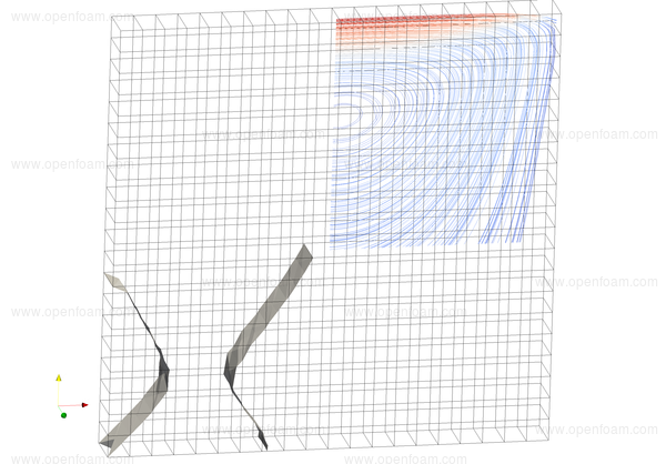
In addition, the resulting surfaces are now constructed with a consistent orientation where the normals of the new triangles point in the direction of an increasing iso-value. The picture below shows an example of clipping the streamlines and iso-surfaces for the lid-driven cavity tutorial case.

Source code

FunctionObject and sampledSurface - $FOAM_/SRC/sampling/sampledSurface/isoSurface
$FOAM_/SRC//postProcessing/functionObjects/fields/streamline
$FOAM_/SRC/postProcessing/functionObjects/field/wallBoundedStreamLine

Ensight surface writer updates

Many function objects and sampling utilities are able to export field data. In earlier versions of OpenFOAM, the surface data file contained both the geometry and field data. For transient data output, this leads to the geometry being written multiple times, even if it remains static.

In this release, surfaceWriter with Ensight format has been re-written to allow the geometry to be written only once. To enable this feature, a new option collateTimes has been added.

The option can be used whenever a generic surface writer is used:

• sample utility
• surfaces function object
• faceSource function object
• FacePostProcessing cloud function object
• ParticleCollector cloud function object

It is specified in the Ensight sub-dictionary of the formatOptions dictionary, employed by the surface writers:

Source code

Ensight surface writer - $FOAM_/SRC/sampling/sampledSurface/writers/ensight

Forces and force coefficients

The forces and forceCoeffs function objects have been updated to enable users to output the force, moment and coefficient data on the boundary field of a volume field. When activated, the fields will be written to the time directories alongside the solver output fields.

The additional field writing is achieved by selecting the new optional user entry writeFields, as shown in the example below:

This will generate the additional (vector) fields in the time directories:

• <functionObjectName>:force
• <functionObjectName>:moment
• <functionObjectName>:forceCoeffs
• <functionObjectName>:momentCoeffs

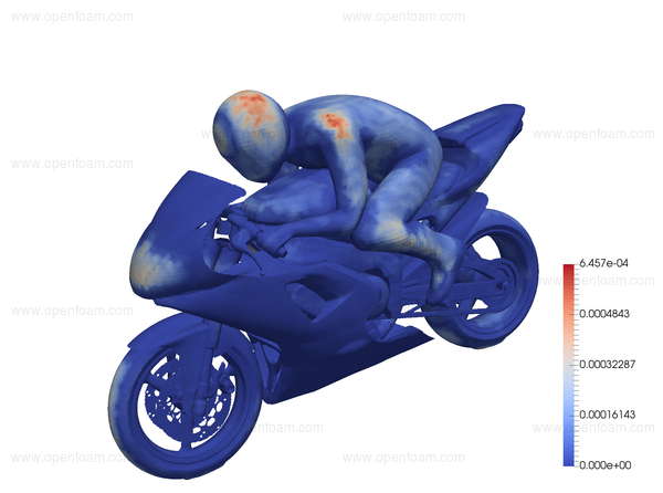
The following image shows an example of the force coefficient output on the surface of the motorBike tutorial:

Source code

Forces - $FOAM_SRC/postProcessing/functionObjects/utilities/forces

PatchProbe Snapping if outside

In OpenFOAM there are two methods to extract patch-based data: using the patchProbes functionObject or using the patchSeed set sampling method (available through the sample utility or functionObject). In the patchProbes functionality the actual location being sampled is the nearest point to the user-provided sampling location. In this release the patchProbes functionObject has been extended to output the actual sampling location instead of the user-provided location.

Secondly the patchSeed set sampling method has been extended to allow the use of user-provided set of points to have similar functionality (Note that compared to the patchProbes method the patchSeed method has the benefit of allowing a user-provided interpolation and write method)

A new keyword points allows sub-setting of the set of patch faces to sample. It can be combined with the limiting of the number of points:

The example above will find for each point in points list, the nearest patch face and sample its face centre.

Source code

PatchSeed $FOAM_SRC/sampling/sampledSet/patchSeed

Generating flow statistics across face zones

The new fluxSummary function object provides flow statistics across face zones, initially added for generating heat exchanger performance data.

Current outputs include the sum of:

• positive fluxes
• negative fluxes
• net fluxes (positive + negative)
• absolute flux (positive - negative)

The set of faces to process are defined by a mode entry, having the options:

• faceZone: process a face zone where the positive direction is given by the face normals
• faceZoneAndDirection: process a face zone where the positive direction specified
• cellZoneAndDirection: extract the surface of a cell zone to generate a set of faces, where the positive direction is given by the face normals

Source code

Forces - $FOAM_SRC/postProcessing/functionObjects/utilities/fluxSummary

Function objects updates

In this release, efforts have been undertaken to standardise the way in which users interact with function objects, with the purposes of presenting a consistent set of inputs to users, and to improve code maintainability and sustainability.

New state dictionary

A new class has been written to maintain function object state information in a dictionary format. This serves as a central database which can be used to exchange information between the objects. For example, to take the output of an object as an input to another object. The state dictionary is written at simulation output times to the $FOAM_/CASE/<time>/uniform/functionObjects/functionObjectProperties directory to ensure consistent restart behaviour.

Header documentation updates The header documentation has been updated and expanded, including updates to:

• $FOAM_SRC/postProcessing/functionObjects/forces
• $FOAM_SRC/postProcessing/functionObjects/fvTools

This information is readily accessible via the Doxygen documentation system, e.g. as invoked via a browser or the foamHelp utility.

Writing data to file

The functionObjectFile base class provides functionality to write function object data to file An additional, optional boolean entry, given by the keyword writeToFile has been added to activate/suppress writing to file, which has a default value of true. Writing data to the standard output efforts have been undertaken to unify the output messages a log keyword can be used to activate/suppress writing to the standard output.

Result name

A new optional entry, resultName, has been added to the family of utility function objects, enabling users to prescribe the name of the result, e.g.:

PressureTools1
{
    type            pressureTools;
    functionObjectLibs ("libutilityFunctionObjects.so");
    ...
    calcTotal       no;
    calcCoeff       yes;

    // Specify optional result name
    resultName      pCoeff;
}

New function objects

valueAverage: takes value(s) from the state dictionary and calculates the ensemble/time average, e.g.: to perform an average of the values output from the forceCoeffs function object.

Functionality updates

The following function objects have been updated:

• pressureTools: in earlier versions of OpenFOAM, a pressure derived from the kinematic pressure () would be zero if the reference density was not set. A check has been implemented to ensure that the reference density is set if needed, avoiding false results.
• faceSource: Improved parallel behaviour by no longer combining source fields onto the master process. Operations involving fluxes (e.g. ) should now use the orientedFields and orientedWeightField options
• cellSource: Improved parallel behaviour by no longer combining source fields onto the master process
• fieldValueDelta: Earlier versions of the object could only operate on fields with the same name, e.g.: . This has been updated to allow operations based on the general field type,e.g. scalar, vector, tensor etc.
• Lambda2: Default name includes the name of the velocity field if it is not , e.g.: Lambda2(UMean)
• Q: Default name includes the name of the velocity field if it is not , e.g.: Q(UMean)
• vorticity: Default name includes the name of the velocity field if it is not , e.g.. vorticity(UMean)

Investigating cells for blended interpolating scheme

The blendingFactor function object generates an indicator field to show which scheme of a blended interpolation is active across the mesh. Whilst this is useful to interrogate local mesh regions, general statistics which reflect the number of cells employed by each each scheme can be useful to asses mesh quality and numerical performance.

For this, the blendingFactor function object has been updated to output the number of cells in each category (first scheme, second scheme, blended):

The usage of function object remains unchanged.

Source code

Blending Factor - $FOAM_/SRC/postProcessing/functionObjects/utilities/blendingFactor