7.1 paraFoam
Post-processing OpenFOAM cases with ParaView is supported in several ways:
- visualise the OpenFOAMblockMeshDict file within ParaView using the PVblockMeshReader module supplied with OpenFOAM.
- read the OpenFOAM data within ParaView using the native ParaView reader for OpenFOAM.
- read the OpenFOAM data within ParaView using the PVFoamReader module supplied with OpenFOAM.
- convert OpenFOAM data to VTK format with the foamToVTK utility.
- generate VTK format during the simulation with the vtkWrite function object. This functionality largely mirrors that of the foamToVTK utility.
- generate output during the simulation by using VTK via the runTimePostProcessing function object.
The main post-processing tool provided with OpenFOAM is ParaView, an open-source visualization application. The most recent ParaView version at the time of release was 5.4.0, which is also the recommended version. Further details about ParaView can be found at http://www.paraview.org and further documentation is available at http://www.kitware.com/products/books/paraview.html.
7.1.1 Overview of paraFoam
paraFoam is strictly a script that launches ParaView, by default using the reader module supplied with OpenFOAM. The term paraFoam may thus sometimes be used synonymously for the OpenFOAM reader module itself. Like any OpenFOAM utility, paraFoam can be executed from within the case directory or with the -case option with the case path as an argument, e.g.:
paraFoam -case <caseDir>
The paraFoam script can conveniently be used to select the PVFoamReader (this is the default behaviour), to select the PVblockMeshReader (using the -block option), or to select the native ParaView reader (using the -vtk option).
7.1.1.1 Recommendations
- The PVblockMeshReader module (paraFoam with -block) is currently the only option visualising the blockMeshDict.
- The native ParaView reader for OpenFOAM (paraFoam with -vtk) is generally the preferred method for general visualisation. It manages decomposed cases and can be used in parallel. However, it understandably does not cope well with complex dictionary input. For such cases, the best recourse is often to skip the 0 initial conditions directory. OpenCFD Ltd. intends to continue participating in the further development of this reader, with several improvements already have been integrated into the ParaView 5.3.0 and 5.4.0 versions.
- The PVFoamReader module (paraFoam default) supplied with OpenFOAM, which predates the native reader, continues to receive active development effort. However, it must be noted the reader only manages serial or reconstructed cases, but does support some features not yet found in native reader (e.g., display of patch names, display of fields per cell-zone…). The primary focus of this reader module is now shifted to support things that the native reader does not, and to serve as a platform for testing new ideas and features.
7.1.2 Converting to VTK format
As an alternative, the OpenFOAM data can be also be converted into VTK format using the foamToVTK utility or during the simulation with the the vtkWrite function object that largely mirrors the functionality of the foamToVTK utility. The converted data can be post-processed in ParaView or any other program supporting VTK format.
Both the foamToVTK utility and the vtkWrite function object support legacy and xml VTK formats.
See the tutorials/incompressible/simpleFoam/windAroundBuildings for an example.
7.1.3 Overview of ParaView
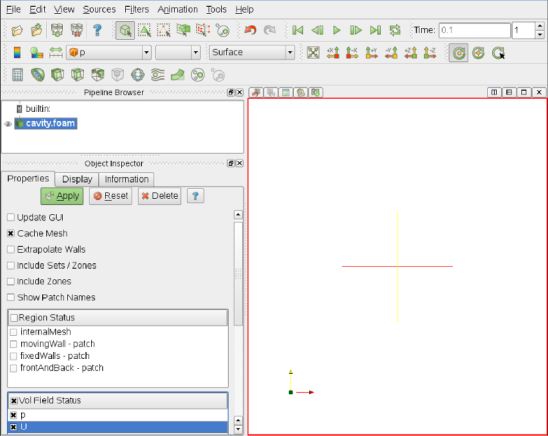
After ParaView is launched and opens, the window shown in Figure 7.1 is displayed. The case is controlled from the left panel, which contains the following:
- Pipeline Browser
- lists the modules opened in ParaView, where the selected modules are highlighted in blue and the graphics for the given module can be enabled/disabled by clicking the eye button alongside;
- Properties panel
- contains the input selections for the case, such as times, regions and fields;
- Display panel
- controls the visual representation of the selected module, e.g. colours;
- Information panel
- gives case statistics such as mesh geometry and size.
ParaView operates a tree-based structure in which data can be filtered from the top-level case module to create sets of sub-modules. For example, a contour plot of, say, pressure could be a sub-module of the case module which contains all the pressure data. The strength of ParaView is that the user can create a number of sub-modules and display whichever ones they feel to create the desired image or animation. For example, they may add some solid geometry, mesh and velocity vectors, to a contour plot of pressure, switching any of the items on and off as necessary.
The general operation of the system is based on the user making a selection and then clicking the green Apply button in the Properties panel. The additional buttons are: the Reset button which is used to reset the GUI if necessary; and, the Delete button that will delete the active module.
7.1.4 The Properties panel
The Properties panel for the case module contains the settings for time step, regions and fields.
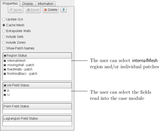
The controls are described in Figure 7.2. It is particularly worth noting that in the current reader module, data in all time directories are loaded into ParaView (in the reader module for ParaView 4.4.0, a set of check boxes controlled the time that were displayed). In the current reader module, the buttons in the Current Time Controls and VCR Controls toolbars select the time data to be displayed, as shown is section 7.1.6.
As with any operation in paraFoam, the user must click Apply after making any changes to any selections. The Apply button is highlighted in green to alert the user if changes have been made but not accepted. This method of operation has the advantage of allowing the user to make a number of selections before accepting them, which is particularly useful in large cases where data processing is best kept to a minimum.
There are occasions when the case data changes on file and ParaView needs to load the changes, e.g. when field data is written into new time directories. To load the changes, the user should check the Update GUI button at the top of the Properties panel and then apply the changes.
7.1.5 The Display panel
The Display panel contains the settings for visualising the data for a given case module.
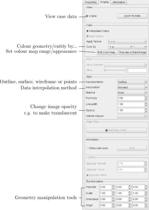
The following points are particularly important:
- the data range may not be automatically updated to the max/min limits of a field, so the user should take care to select Rescale to Data Range at appropriate intervals, in particular after loading the initial case module;
- clicking the Edit Color Map button, brings up a window in which there are
two panels:
- The Color Scale panel in which the colours within the scale can be chosen. The standard blue to red colour scale for CFD can be selected by clicking Choose Preset and selecting Blue to Red Rainbox HSV.
- The Color Legend panel has a toggle switch for a colour bar legend and contains settings for the layout of the legend, e.g. font.
- the underlying mesh can be represented by selecting Wireframe in the Representation menu of the Style panel;
- the geometry, e.g. a mesh (if Wireframe is selected), can be visualised as a single colour by selecting Solid Color from the Color By menu and specifying the colour in the Set Ambient Color window;
- the image can be made translucent by editing the value in the Opacity text box (1 = solid, 0 = invisible) in the Style panel.
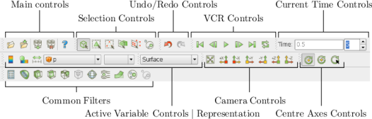
7.1.6 The button toolbars
ParaView duplicates functionality from pull-down menus at the top of the main window and the major panels, within the toolbars below the main pull-down menus. The displayed toolbars can be selected from Toolbars in the main View menu. The default layout with all toolbars is shown in Figure 7.4 with each toolbar labelled. The function of many of the buttons is clear from their icon and, with tooltips enabled in the Help menu, the user is given a concise description of the function of any button.
7.1.7 Manipulating the view
This section describes operations for setting and manipulating the view of objects in paraFoam.
7.1.7.1 View settings
The View Settings are selected from the Edit menu, which opens a View Settings (Render View) window with a table of 3 items: General, Lights and Annotation. The General panel includes the following items which are often worth setting at startup:
- the background colour, where white is often a preferred choice for printed material, is set by choosing background from the down-arrow button next to Choose Color button, then selecting the color by clicking on the Choose Color button;
- Use parallel projection which is the usual choice for CFD, especially for 2D cases.
The Lights panel contains detailed lighting controls within the Light Kit panel. A separate Headlight panel controls the direct lighting of the image. Checking the Headlight button with white light colour of strength 1 seems to help produce images with strong bright colours, e.g. with an isosurface.
The Annotation panel includes options for including annotations in the image.
The Orientation Axes feature controls an axes icon in the image window, e.g. to set
the colour of the axes labels  ,
,  and
and  .
.
7.1.7.2 General settings
The general Settings are selected from the Edit menu, which opens a general Options window with General, Colors, Animations, Charts and Render View menu items.
The General panel controls some default behaviour of ParaView. In particular, there is an Auto Accept button that enables ParaView to accept changes automatically without clicking the green Apply button in the Properties window. For larger cases, this option is generally not recommended: the user does not generally want the image to be re-rendered between each of a number of changes he/she selects, but be able to apply a number of changes to be re-rendered in their entirety once.
The Render View panel contains 3 sub-items: General, Camera and Server. The General panel includes the level of detail (LOD) which controls the rendering of the image while it is being manipulated, e.g. translated, resized, rotated; lowering the levels set by the sliders, allows cases with large numbers of cells to be re-rendered quickly during manipulation.
The Camera panel includes control settings for 3D and 2D movements. This presents the user with a map of rotation, translate and zoom controls using the mouse in combination with Shift- and Control-keys. The map can be edited to suit by the user.
7.1.8 Contour plots
A contour plot is created by selecting Contour from the Filter menu at the top menu bar. The filter acts on a given module so that, if the module is the 3D case module itself, the contours will be a set of 2D surfaces that represent a constant value, i.e. isosurfaces. The Properties panel for contours contains an Isosurfaces list that the user can edit, most conveniently by the New Range window. The chosen scalar field is selected from a pull down menu.
7.1.8.1 Introducing a cutting plane
Very often a user will wish to create a contour plot across a plane rather than producing isosurfaces. To do so, the user must first use the Slice filter to create the cutting plane, on which the contours can be plotted. The Slice filter allows the user to specify a cutting Plane, Box or Sphere in the Slice Type menu by a center and normal/radius respectively. The user can manipulate the cutting plane like any other using the mouse.
The user can then run the Contour filter on the cut plane to generate contour lines.
7.1.9 Vector plots
Vector plots are created using the Glyph filter. The filter reads the field selected in Vectors and offers a range of Glyph Types for which the Arrow provides a clear vector plot images. Each glyph has a selection of graphical controls in a panel which the user can manipulate to best effect.
The remainder of the Properties panel contains mainly the Scale Mode menu for the glyphs. The most common options are Scale Mode are: Vector, where the glyph length is proportional to the vector magnitude; and, Off where each glyph is the same length. The Set Scale Factor parameter controls the base length of the glyphs.
7.1.9.1 Plotting at cell centres
Vectors are by default plotted on cell vertices but, very often, we wish to plot data at cell centres. This is done by first applying the Cell Centers filter to the case module, and then applying the Glyph filter to the resulting cell centre data.
7.1.10 Streamlines
Streamlines are created by first creating tracer lines using the Stream Tracer filter. The tracer Seed panel specifies a distribution of tracer points over a Line Source or Point Cloud. The user can view the tracer source, e.g. the line, but it is displayed in white, so they may need to change the background colour in order to see it.
The distance the tracer travels and the length of steps the tracer takes are specified in the text boxes in the main Stream Tracer panel. The process of achieving desired tracer lines is largely one of trial and error in which the tracer lines obviously appear smoother as the step length is reduced but with the penalty of a longer calculation time.
Once the tracer lines have been created, the Tubes filter can be applied to the Tracer module to produce high quality images. The tubes follow each tracer line and are not strictly cylindrical but have a fixed number of sides and given radius. When the number of sides is set above, say, 10, the tubes do however appear cylindrical, but again this adds a computational cost.
7.1.11 Image output
The simplest way to output an image to file from ParaView is to select Save
Screenshot from the File menu. On selection, a window appears in which the
user can select the resolution for the image to save. There is a button that, when
clicked, locks the aspect ratio, so if the user changes the resolution in one
direction, the resolution is adjusted in the other direction automatically. After
selecting the pixel resolution, the image can be saved. To achieve high quality
output, the user might try setting the pixel resolution to 1000 or more in the
 -direction so that when the image is scaled to a typical size of a figure in an A4
or US letter document, perhaps in a PDF document, the resolution is
sharp.
-direction so that when the image is scaled to a typical size of a figure in an A4
or US letter document, perhaps in a PDF document, the resolution is
sharp.
7.1.12 Animation output
To create an animation, the user should first select Save Animation from the File menu. A dialogue window appears in which the user can specify a number of things including the image resolution. The user should specify the resolution as required. The other noteworthy setting is number of frames per timestep. While this would intuitively be set to 1, it can be set to a larger number in order to introduce more frames into the animation artificially. This technique can be particularly useful to produce a slower animation because some movie players have limited speed control, particularly over mpeg movies.
On clicking the Save Animation button, another window appears in which the user specifies a file name root and file format for a set of images. On clicking OK, the set of files will be saved according to the naming convention “<fileRoot>_<imageNo>.<fileExt>”, e.g. the third image of a series with the file root “animation”, saved in jpg format would be named “animation_0002.jpg” (<imageNo> starts at 0000).
Once the set of images are saved the user can convert them into a movie using their software of choice. The convert utility in the ImageMagick package can do this from the command line, e.g. by
convert animation*jpg movie.mpg