3.3 Decompression of a tank internally pressurised with water
Tutorial path:
In this example we shall investigate a problem of rapid opening of a pipe valve close to a pressurised liquid-filled tank. The prominent feature of the result in such cases is the propagation of pressure waves which must therefore be modelled as a compressible liquid.
This tutorial introduces the following OpenFOAM features for the first time:
3.3.1 Problem specification
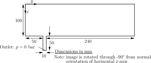
- Solution domain
- The domain is 2 dimensional and consists of
a tank with a small outflow pipe as shown in Figure 3.6
- Governing equations
- This problem requires a model for compressibility
 in
the fluid in order to be able to resolve waves propagating at a finite speed. A
barotropic relationship is used to relate density
in
the fluid in order to be able to resolve waves propagating at a finite speed. A
barotropic relationship is used to relate density  and pressure
  are
related to
are
related to  .
.
- Mass continuity
(3.11) - The barotropic relationship

(3.12) where
 is the bulk modulus
- Equation 3.12 is linearised as
(3.13) where
 and
and  are the reference density and pressure respectively
such that
are the reference density and pressure respectively
such that  .
.
- Momentum equation for Newtonian fluid
(3.14)
- Mass continuity
- Boundary conditions
- Initial conditions
 ,
,  .
.
- Transport properties
-
- Dynamic viscosity of water

- Dynamic viscosity of water
- Thermodynamic properties
-
- Density of water
- Reference pressure

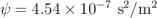
- Compressibility of water
- Density of water
- Solver name
- sonicLiquidFoam: a solver for compressible sonic laminar liquid flow.
- Case name
- decompressionTank case located in the $FOAM_TUTORIALS/compressible/sonicLiquidFoam directory.
 bar.
bar.
3.3.2 Mesh Generation
The full geometry is modelled in this case; the set of vertices and blocks are given in the mesh description file below:
1/*--------------------------------*- C++ -*----------------------------------*\
2| ========= | |
3| \\ / F ield | OpenFOAM: The Open Source CFD Toolbox |
4| \\ / O peration | Version: v2006 |
5| \\ / A nd | Website: www.openfoam.com |
6| \\/ M anipulation | |
7\*---------------------------------------------------------------------------*/
8FoamFile
9{
10 version 2.0;
11 format ascii;
12 class dictionary;
13 object blockMeshDict;
14}
15// * * * * * * * * * * * * * * * * * * * * * * * * * * * * * * * * * * * * * //
16
17scale 0.1;
18
19vertices
20(
21 (0 0 -0.1)
22 (1 0 -0.1)
23 (0 0.5 -0.1)
24 (1 0.5 -0.1)
25 (1.5 0.5 -0.1)
26 (0 0.6 -0.1)
27 (1 0.6 -0.1)
28 (1.5 0.6 -0.1)
29 (0 3 -0.1)
30 (1 3 -0.1)
31 (0 0 0.1)
32 (1 0 0.1)
33 (0 0.5 0.1)
34 (1 0.5 0.1)
35 (1.5 0.5 0.1)
36 (0 0.6 0.1)
37 (1 0.6 0.1)
38 (1.5 0.6 0.1)
39 (0 3 0.1)
40 (1 3 0.1)
41);
42
43blocks
44(
45 hex (0 1 3 2 10 11 13 12) (30 20 1) simpleGrading (1 1 1)
46 hex (2 3 6 5 12 13 16 15) (30 5 1) simpleGrading (1 1 1)
47 hex (3 4 7 6 13 14 17 16) (25 5 1) simpleGrading (1 1 1)
48 hex (5 6 9 8 15 16 19 18) (30 95 1) simpleGrading (1 1 1)
49);
50
51edges
52(
53);
54
55boundary
56(
57 outerWall
58 {
59 type wall;
60 faces
61 (
62 (0 1 11 10)
63 (1 3 13 11)
64 (3 4 14 13)
65 (7 6 16 17)
66 (6 9 19 16)
67 (9 8 18 19)
68 );
69 }
70 axis
71 {
72 type symmetryPlane;
73 faces
74 (
75 (0 10 12 2)
76 (2 12 15 5)
77 (5 15 18 8)
78 );
79 }
80 nozzle
81 {
82 type patch;
83 faces
84 (
85 (4 7 17 14)
86 );
87 }
88 back
89 {
90 type empty;
91 faces
92 (
93 (0 2 3 1)
94 (2 5 6 3)
95 (3 6 7 4)
96 (5 8 9 6)
97 );
98 }
99 front
100 {
101 type empty;
102 faces
103 (
104 (10 11 13 12)
105 (12 13 16 15)
106 (13 14 17 16)
107 (15 16 19 18)
108 );
109 }
110);
111
112mergePatchPairs
113(
114);
115
116// ************************************************************************* //
In order to improve the numerical accuracy, we shall use the reference level of
1  for the pressure field. Note that both the internal field level and the
boundary conditions are offset by the reference level.
for the pressure field. Note that both the internal field level and the
boundary conditions are offset by the reference level.
3.3.3 Preparing the Run
Before we commence the setup of the calculation, we need to consider the characteristic velocity of the phenomenon we are trying to capture. In the case under consideration, the fluid velocity will be very small, but the pressure wave will propagate with the speed of sound in water. The speed of sound is calculated as:
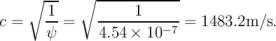 | (3.15) |
For the mesh described above, the characteristic mesh size is approximately
2  (note the scaling factor of
  in the blockMeshDict file). Using
 | (3.16) |
a reasonable time step is around  , giving the
  number of
 , based on the speed of sound. Also, note that the reported
  number by
the code (associated with the convective velocity) will be two orders of magnitude
smaller. As we are interested in the pressure wave propagation, we shall set the
simulation time to
number by
the code (associated with the convective velocity) will be two orders of magnitude
smaller. As we are interested in the pressure wave propagation, we shall set the
simulation time to  . For reference, the controlDict file is quoted
below.
. For reference, the controlDict file is quoted
below.
1/*--------------------------------*- C++ -*----------------------------------*\
2| ========= | |
3| \\ / F ield | OpenFOAM: The Open Source CFD Toolbox |
4| \\ / O peration | Version: v2006 |
5| \\ / A nd | Website: www.openfoam.com |
6| \\/ M anipulation | |
7\*---------------------------------------------------------------------------*/
8FoamFile
9{
10 version 2.0;
11 format ascii;
12 class dictionary;
13 location "system";
14 object controlDict;
15}
16// * * * * * * * * * * * * * * * * * * * * * * * * * * * * * * * * * * * * * //
17
18application sonicLiquidFoam;
19
20startFrom startTime;
21
22startTime 0;
23
24stopAt endTime;
25
26endTime 0.0001;
27
28deltaT 5e-07;
29
30writeControl timeStep;
31
32writeInterval 20;
33
34purgeWrite 0;
35
36writeFormat ascii;
37
38writePrecision 6;
39
40writeCompression off;
41
42timeFormat general;
43
44timePrecision 6;
45
46runTimeModifiable true;
47
48
49// ************************************************************************* //
3.3.4 Running the case
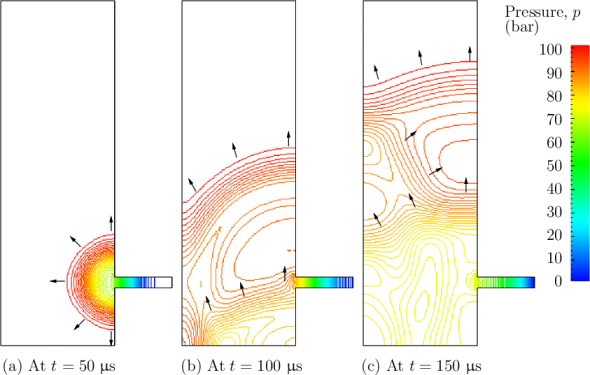
The user can run the case and view results in dxFoam. The liquid flows out through the nozzle causing a wave to move along the nozzle. As it reaches the inlet to the tank, some of the wave is transmitted into the tank and some of it is reflected. While a wave is reflected up and down the inlet pipe, the waves transmitted into the tank expand and propagate through the tank. In Figure 3.7, the pressures are shown as contours so that the wave fronts are more clearly defined than if plotted as a normal isoline plot.
If the simulation is run for a long enough time for the reflected wave to return to the pipe, we can see that negative absolute pressure is detected. The modelling permits this and has some physical basis since liquids can support tension, i.e. negative pressures. In reality, however, impurities or dissolved gases in liquids act as sites for cavitation, or vapourisation/boiling, of the liquid due to the low pressure. Therefore in practical situations, we generally do not observe pressures falling below the vapourisation pressure of the liquid; not at least for longer than it takes for the cavitation process to occur.
3.3.5 Improving the solution by refining the mesh
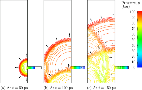
Looking at the evolution of the resulting pressure field in time, we can clearly
see the propagation of the pressure wave into the tank and numerous reflections
from the inside walls. It is also obvious that the pressure wave is smeared over a
number of cells. We shall now refine the mesh and reduce the time step to obtain
a sharper front resolution. Simply edit the blockMeshDict and increase the number
of cells by a factor of 4 in the  and
and  directions, i.e. block 0 becomes
(120 80 1) from (30 20 1) and so on. Run blockMesh on this file. In
addition, in order to maintain a Courant number below 1, the time step
must be reduced accordingly to
directions, i.e. block 0 becomes
(120 80 1) from (30 20 1) and so on. Run blockMesh on this file. In
addition, in order to maintain a Courant number below 1, the time step
must be reduced accordingly to  . The second simulation
gives considerably better resolution of the pressure waves as shown in
Figure 3.8.
. The second simulation
gives considerably better resolution of the pressure waves as shown in
Figure 3.8.