3.1 Steady turbulent flow over a backward-facing step
Tutorial path:
In this example we shall investigate steady turbulent flow over a backward-facing step. The problem description is taken from one used by Pitz and Daily in an experimental investigation [**] against which the computed solution can be compared. This example introduces the following OpenFOAM features for the first time:
3.1.1 Problem specification
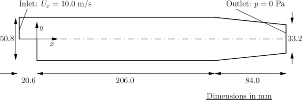
The problem is defined as follows:
- Solution domain
- The domain is 2 dimensional, consisting of a short inlet, a
backward-facing step and converging nozzle at outlet as shown in Figure 3.1.
- Governing equations
- Initial conditions
 ,
,  — required in OpenFOAM
input files but not necessary for the solution since the problem is
steady-state.
— required in OpenFOAM
input files but not necessary for the solution since the problem is
steady-state.
- Boundary conditions
-
- Inlet (left) with fixed velocity
 m/s;
m/s;
- Outlet (right) with fixed pressure
 ;
;
- No-slip walls on other boundaries.
- Inlet (left) with fixed velocity
- Transport properties
-
- Kinematic viscosity of air

- Kinematic viscosity of air
- Turbulence model
-
- Standard
 ;
;
- Coefficients:
 .
.
- Standard
- Solver name
- simpleFoam: an implementation for steady incompressible flow.
- Case name
- pitzDaily, located in the $FOAM_TUTORIALS/incompressible/simpleFoam directory.

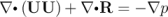
 is kinematic pressure and (in slightly over-simplistic terms)
 is the viscous stress term with an effective kinematic
viscosity
is the viscous stress term with an effective kinematic
viscosity  , calculated from selected transport and turbulence
models.
, calculated from selected transport and turbulence
models.The problem is solved using simpleFoam, so-called as it is an implementation for steady flow using the SIMPLE algorithm. The solver has full access to all the turbulence models in the incompressibleTurbulenceModels library and the non-Newtonian models incompressibleTransportModels library of the standard OpenFOAM release.
3.1.2 Mesh generation
We expect that the flow in this problem is reasonably complex and an
optimum solution will require grading of the mesh. In general, the regions of
highest shear are particularly critical, requiring a finer mesh than in the
regions of low shear. We can anticipate where high shear will occur by
considering what the solution might be in advance of any calculation.
At the inlet we have strong uniform flow in the  direction and, as it
passes over the step, it generates shear on the fluid below, generating
a vortex in the bottom half of the domain. The regions of high shear
will therefore be close to the centreline of the domain and close to the
walls.
direction and, as it
passes over the step, it generates shear on the fluid below, generating
a vortex in the bottom half of the domain. The regions of high shear
will therefore be close to the centreline of the domain and close to the
walls.
The domain is subdivided into 12 blocks as shown in Figure 3.2.
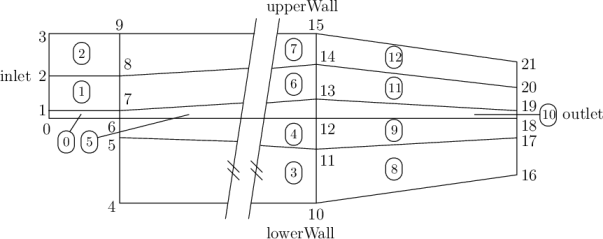
The mesh is 3 dimensional, as always in OpenFOAM, so in Figure 3.2 we are
viewing the back plane along  . The full set of vertices and blocks are
given in the mesh description file below:
. The full set of vertices and blocks are
given in the mesh description file below:
1/*--------------------------------*- C++ -*----------------------------------*\
2| ========= | |
3| \\ / F ield | OpenFOAM: The Open Source CFD Toolbox |
4| \\ / O peration | Version: v2006 |
5| \\ / A nd | Website: www.openfoam.com |
6| \\/ M anipulation | |
7\*---------------------------------------------------------------------------*/
8FoamFile
9{
10 version 2.0;
11 format ascii;
12 class dictionary;
13 object blockMeshDict;
14}
15// * * * * * * * * * * * * * * * * * * * * * * * * * * * * * * * * * * * * * //
16
17scale 0.001;
18
19vertices
20(
21 (-20.6 0 -0.5)
22 (-20.6 25.4 -0.5)
23 (0 -25.4 -0.5)
24 (0 0 -0.5)
25 (0 25.4 -0.5)
26 (206 -25.4 -0.5)
27 (206 0 -0.5)
28 (206 25.4 -0.5)
29 (290 -16.6 -0.5)
30 (290 0 -0.5)
31 (290 16.6 -0.5)
32
33 (-20.6 0 0.5)
34 (-20.6 25.4 0.5)
35 (0 -25.4 0.5)
36 (0 0 0.5)
37 (0 25.4 0.5)
38 (206 -25.4 0.5)
39 (206 0 0.5)
40 (206 25.4 0.5)
41 (290 -16.6 0.5)
42 (290 0 0.5)
43 (290 16.6 0.5)
44);
45
46negY
47(
48 (2 4 1)
49 (1 3 0.3)
50);
51
52posY
53(
54 (1 4 2)
55 (2 3 4)
56 (2 4 0.25)
57);
58
59posYR
60(
61 (2 1 1)
62 (1 1 0.25)
63);
64
65
66blocks
67(
68 hex (0 3 4 1 11 14 15 12)
69 (18 30 1)
70 simpleGrading (0.5 $posY 1)
71
72 hex (2 5 6 3 13 16 17 14)
73 (180 27 1)
74 edgeGrading (4 4 4 4 $negY 1 1 $negY 1 1 1 1)
75
76 hex (3 6 7 4 14 17 18 15)
77 (180 30 1)
78 edgeGrading (4 4 4 4 $posY $posYR $posYR $posY 1 1 1 1)
79
80 hex (5 8 9 6 16 19 20 17)
81 (25 27 1)
82 simpleGrading (2.5 1 1)
83
84 hex (6 9 10 7 17 20 21 18)
85 (25 30 1)
86 simpleGrading (2.5 $posYR 1)
87);
88
89edges
90(
91);
92
93boundary
94(
95 inlet
96 {
97 type patch;
98 faces
99 (
100 (0 1 12 11)
101 );
102 }
103 outlet
104 {
105 type patch;
106 faces
107 (
108 (8 9 20 19)
109 (9 10 21 20)
110 );
111 }
112 upperWall
113 {
114 type wall;
115 faces
116 (
117 (1 4 15 12)
118 (4 7 18 15)
119 (7 10 21 18)
120 );
121 }
122 lowerWall
123 {
124 type wall;
125 faces
126 (
127 (0 3 14 11)
128 (3 2 13 14)
129 (2 5 16 13)
130 (5 8 19 16)
131 );
132 }
133 frontAndBack
134 {
135 type empty;
136 faces
137 (
138 (0 3 4 1)
139 (2 5 6 3)
140 (3 6 7 4)
141 (5 8 9 6)
142 (6 9 10 7)
143 (11 14 15 12)
144 (13 16 17 14)
145 (14 17 18 15)
146 (16 19 20 17)
147 (17 20 21 18)
148 );
149 }
150);
151
152// ************************************************************************* //
A major feature of this problem is the use of the full mesh grading
capability of blockMesh that is described in section ?? of the User Guide. The
user can see that blocks 4,5 and 6 use the full list of 12 expansion ratios.
The expansion ratios correspond to each edge of the block, the first 4 to
the edges aligned in the local  direction, the second 4 to the edges
in the local
direction, the second 4 to the edges
in the local  direction and the last 4 to the edges in the local
  direction. In blocks 4, 5, and 6, the ratios are equal for all edges in the local
 and
and  directions but not for the edges in the
  direction that
corresponds in all blocks to the global
direction that
corresponds in all blocks to the global  . If we consider the ratios used
in relation to the block definition in section ?? of the User Guide, we
realize that different gradings have been prescribed along the left and right
edges in blocks 4,5 and 6 in Figure 3.2. The purpose of this differential
grading is to generate a fine mesh close to the most critical region of
flow, the corner of the step, and allow it to expand into the rest of the
domain.
. If we consider the ratios used
in relation to the block definition in section ?? of the User Guide, we
realize that different gradings have been prescribed along the left and right
edges in blocks 4,5 and 6 in Figure 3.2. The purpose of this differential
grading is to generate a fine mesh close to the most critical region of
flow, the corner of the step, and allow it to expand into the rest of the
domain.
The mesh can be generated using blockMesh from the command line and viewed as described in previous examples.
3.1.3 Boundary conditions and initial fields
Edit the case files to set the initial and boundary fields for velocity  , pressure
 , turbulent kinetic energy
  and dissipation rate
  . The boundary conditions
can be specified as: the upper and lower walls are set to Wall, the left
patch to Inlet and the right patch to Outlet. These physical boundary
conditions require us to specify a fixedValue at the inlet on
. The boundary conditions
can be specified as: the upper and lower walls are set to Wall, the left
patch to Inlet and the right patch to Outlet. These physical boundary
conditions require us to specify a fixedValue at the inlet on  ,
,  and
and
 .
.  is given in the problem specification, but the values of
  and
and
 must be chosen by the user in a similar manner to that described in
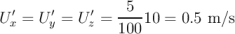
section 2.1.8.1 of the User Guide. We assume that the inlet turbulence is
isotropic and estimate the fluctuations to be
must be chosen by the user in a similar manner to that described in
section 2.1.8.1 of the User Guide. We assume that the inlet turbulence is
isotropic and estimate the fluctuations to be  of
of  at the inlet. We
have
at the inlet. We
have
 | (3.3) |
and
 | (3.4) |
If we estimate the turbulent length scale  to be
to be  of the width of the inlet
then
of the width of the inlet
then
 | (3.5) |
At the outlet we need only specify the pressure  .
.
3.1.4 Case control
The choices of fvSchemes are as follows: the timeScheme should be steadyState; the gradSchemes and laplacianSchemes should be set as default to Gauss; and, the divSchemes should be set to upwind to ensure boundedness.
Special attention should be paid to the solver settings of the fvSolution
dictionary. Although the top level simpleFoam code contains only equations for  and
and  , the turbulence model solves equations for
  ,
,  and
and  , and
tolerance settings are required for all 5 equations. A tolerance of
, and
tolerance settings are required for all 5 equations. A tolerance of  and
relTol of 0.1 are acceptable for all variables with the exception of
and
relTol of 0.1 are acceptable for all variables with the exception of  when
when  and 0.01 are recommended. Under-relaxation of the solution
is required since the problem is steady. A relaxationFactor of 0.7 is
acceptable for
and 0.01 are recommended. Under-relaxation of the solution
is required since the problem is steady. A relaxationFactor of 0.7 is
acceptable for  ,
,  , and
, and  but 0.3 is required for
  to avoid numerical
instability.
to avoid numerical
instability.
Finally, in the controlDict dictionary, the time step deltaT should be set to 1 since in steady state cases such as this is effectively an iteration counter. With benefit of hindsight we know that the solution requires 1000 iterations reach reasonable convergence, hence endTime is set to 1000. Ensure that the writeInterval is sufficiently high, e.g. 50, that you will not fill the hard disk with data during run time.
3.1.5 Running the case and post-processing
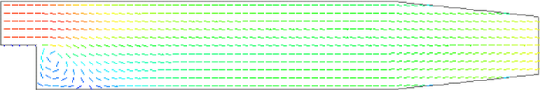
(a) Velocity vectors after 50 iterations |
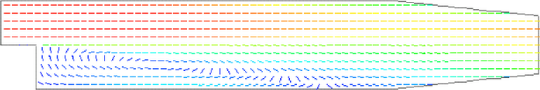
(b) Velocity vectors at 1000 iterations |
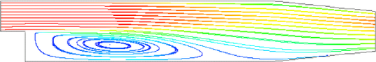
(c) Streamlines at 1000 iterations |
Figure 3.3: Development of a vortex in the backward-facing step.
Run the case and post-process the results. After a few iterations, e.g. 50, a
vortex develops beneath the corner of the step that is the height of the step but
narrow in the  -direction as shown by the vector plot of velocities is
shown Figure 3.3(a). Over several iterations the vortex stretches in the
-direction from the step to the outlet until at 1000 iterations the system
reaches a steady-state in which the vortex is fully developed as shown in
Figure 3.3(b-c).
-direction as shown by the vector plot of velocities is
shown Figure 3.3(a). Over several iterations the vortex stretches in the
-direction from the step to the outlet until at 1000 iterations the system
reaches a steady-state in which the vortex is fully developed as shown in
Figure 3.3(b-c).