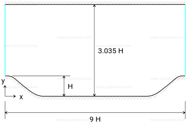
\[ y(x) = \begin{cases} \min(1, a_1 + b_1 x + c_1 x^2 + d_1 x^3) & 0 \le x \lt 9, \\ a_2 + b_2 x + c_2 x^2 + d_2 x^3 & 9 \le x \lt 14, \\ a_3 + b_3 x + c_3 x^2 + d_3 x^3 & 14 \le x \lt 20, \\ a_4 + b_4 x + c_4 x^2 + d_4 x^3 & 20 \le x \lt 30, \\ a_5 + b_5 x + c_5 x^2 + d_5 x^3 & 30 \le x \lt 40, \\ \max(0, a_6 + b_6 x + c_6 x^2 + d_6 x^3) & 40 \le x \lt 54. \\ \end{cases} \]
| a | b | c | d | |
|---|---|---|---|---|
| 1 | \( 28 \) | \( 0 \) | \( 6.775070969851 \times 10^{-3} \) | \( - 2.124527775800 \times 10^{-3} \) |
| 2 | \( 25.07355893131 \times 10^0\) | \( 0.9754803562315 \times 10^{0} \) | \( - 1.016116352781 \times 10^{-1} \) | \( 1.889794677828 \times 10^{-3} \) |
| 3 | \( 2.579601052357 \times 10^1 \) | \( 8.206693007457 \times 10^{-1} \) | \( - 9.055370274339 \times 10^{-2} \) | \( 1.626510569859 \times 10^{-3} \) |
| 4 | \( 4.046435022819 \times 10^1 \) | \( -1.379581654948 \times 10^{0} \) | \( 1.945884504128 \times 10^{-2} \) | \( - 2.070318932190 \times 10^{-4} \) |
| 5 | \( 1.792461334664 \times 10^1 \) | \( 8.743920332081 \times 10^{-1} \) | \( - 5.567361123058 \times 10^{-2} \) | \( 6.277731764683 \times 10^{-4} \) |
| 6 | \( 5.639011190988 \times 10^1 \) | \( -2.010520359035 \times 10^{0} \) | \( 1.644919857549 \times 10^{-2} \) | \( 2.674976141766 \times 10^{-5} \) |
blockMeshDict using a codeStream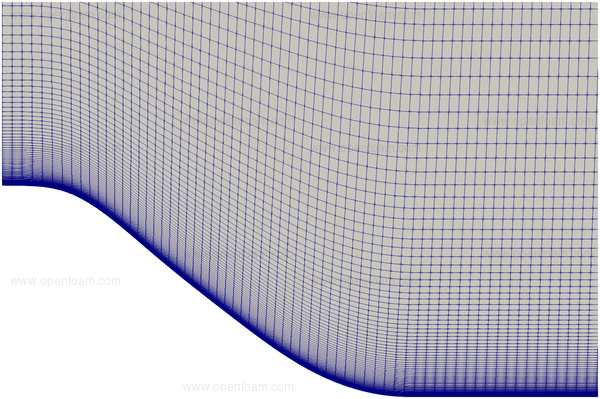
\[ \u_b = \frac{1}{2.0355H}\int\limits_{H}^{3.035H} \u_x (y) dy \]
\[ \nu_\infty = \frac{|\u_b| H}{Re} = \frac{1 \times 0.028}{10565} = 2.65 \times 10^{-6} m^2/s \]
Velocity: U
| Patch | condition | value |
|---|---|---|
| Inlet | cyclic | |
| Outlet | cyclic | |
| Hills | noSlip | |
| Walls | noSlip |
Pressure: p
| Patch | condition | value |
|---|---|---|
| Inlet | cyclic | |
| Outlet | cyclic | |
| Hills | zeroGradient | |
| Walls | zeroGradient |
Turbulence viscosity: nut
| Patch | condition | value |
|---|---|---|
| Inlet | cyclic | |
| Outlet | cyclic | |
| Hills | nutUSpaldingWallFunction | |
| Walls | nutUSpaldingWallFunction |
Modified turbulence viscosity: nuTilda
| Patch | condition | value |
|---|---|---|
| Inlet | cyclic | |
| Outlet | cyclic | |
| Hills | fixedValue | 0 |
| Walls | fixedValue | 0 |
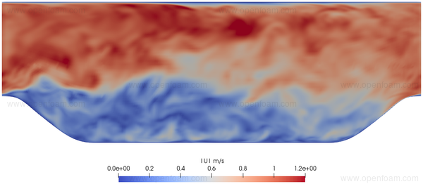
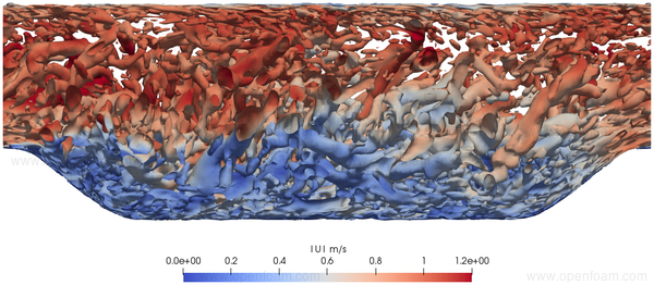
The precursor steady computation is used to initialise the transient calculation. After evolving the transient case for XXX flow-throughs a fully turbulent flow is established, as shown by the instantaneous velocity:
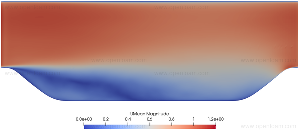
The average velocity prediction shows differences compared to the velocity derived from the precursor steady calculation:
Turbulent structures are clealy evident in the instantanous Q criterion prediction:
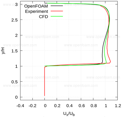
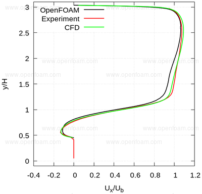
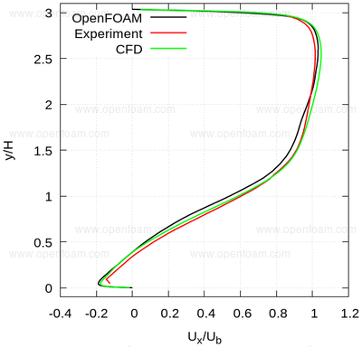
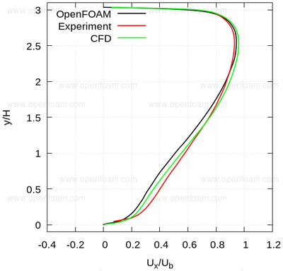
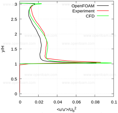
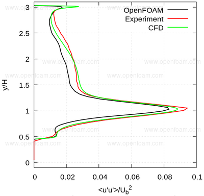
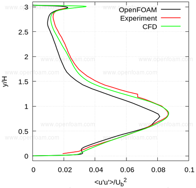
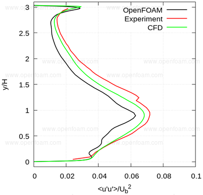
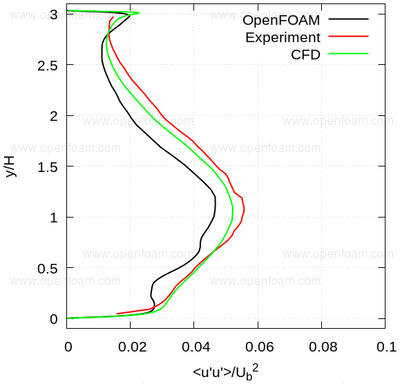
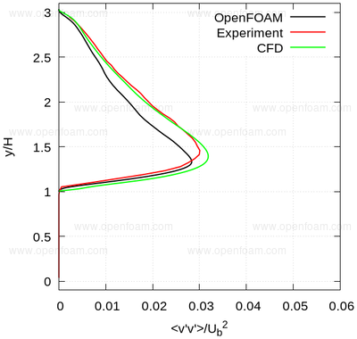
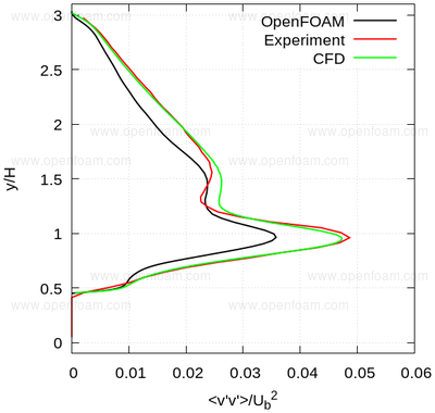
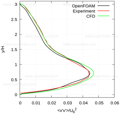
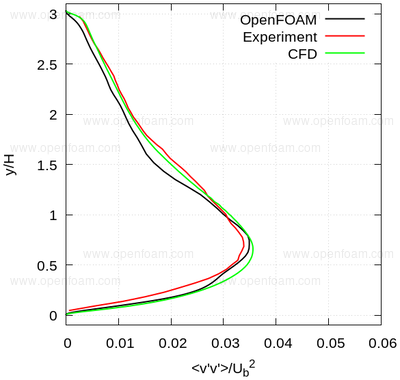
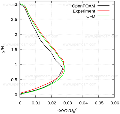
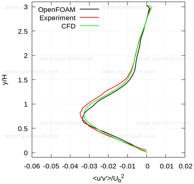
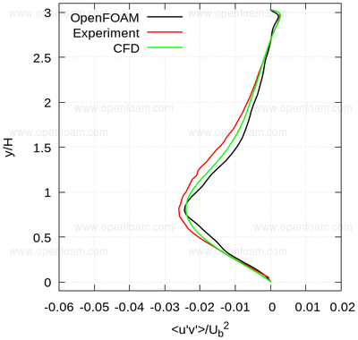
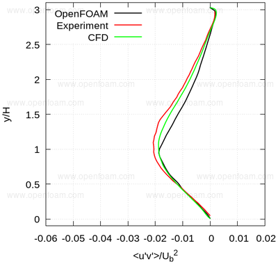
The following series of images provide a quantitative comparison between OpenFOAM predictions and both measured data and results from another CFD code at various streamwise locations.
Average velocity profiles:
U 0.05 | 
U 0.5 |
U 1 | 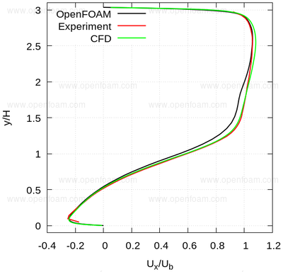
U 2 |
U 3 | 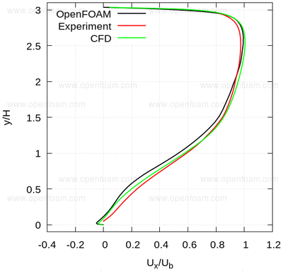
U 4 |

U 5 | 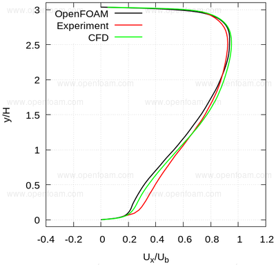
U 6 |
U 7 | 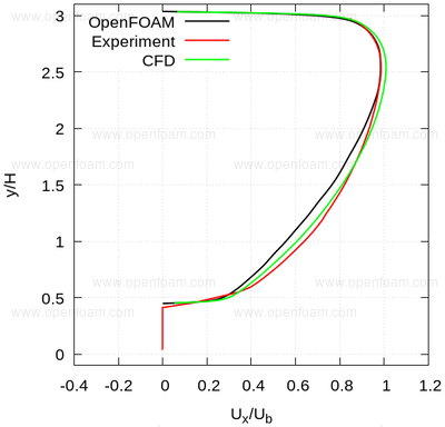
U 8 |
Average normal stresses: uu
uu 0.05 | 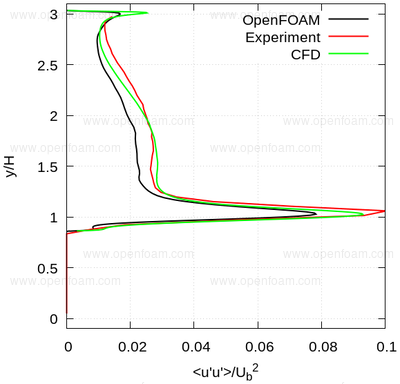
uu 0.5 |
uu 1 | 
uu 2 |
uu 3 | 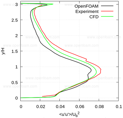
uu 4 |
uu 5 | 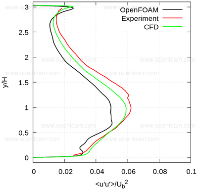
uu 6 |
uu 7 | 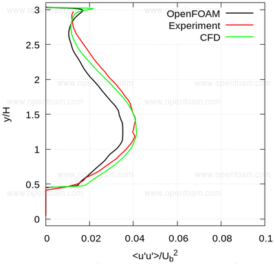
uu 8 |
Average normal stresses: vv
vv 0.05 | 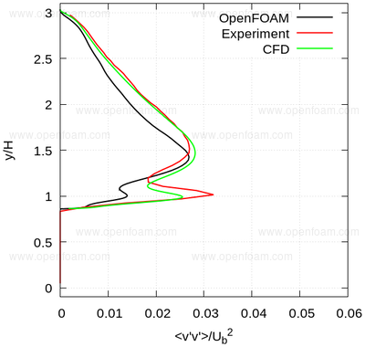
vv 0.5 |
vv 1 | 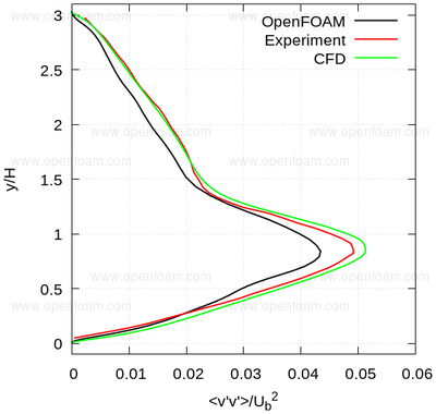
vv 2 |
vv 3 | 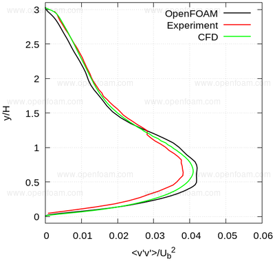
vv 4 |
vv 5 | 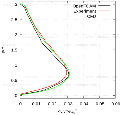
vv 6 |
vv 7 | 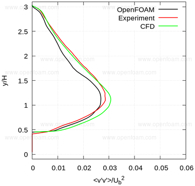
vv 8 |
Average shear stress: uv
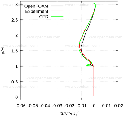
uv 0.05 | 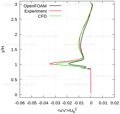
uv 0.5 |
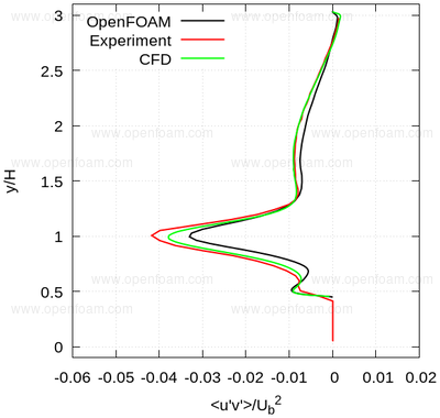
uv 1 | 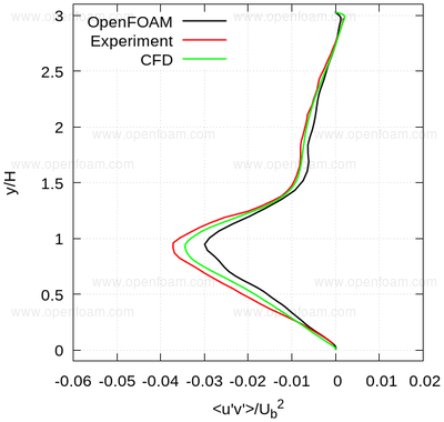
uv 2 |
uv 3 | 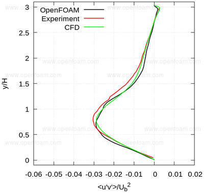
uv 4 |
uv 5 | 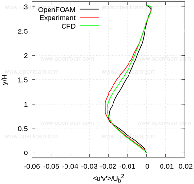
uv 6 |
uv 7 | 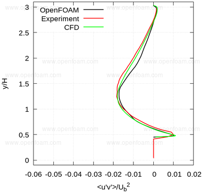
uv 8 |
| Would you like to suggest an improvement to this page? | Create an issue |
Copyright © 2018 OpenCFD Ltd.
Licensed under the Creative Commons License BY-NC-ND 
 1.8.17