Case files can be found here:
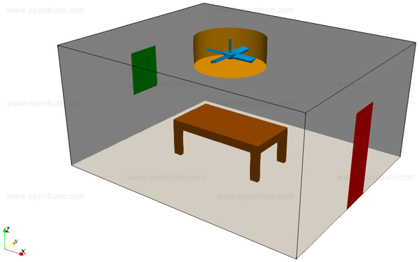
The geometry for this tutorial consists of
The mesh is created with snappyHexMesh using STL surfaces located in the constant/triSurface directory.
surfaceFeatureExtract
The process begins by extracting features from the STL files (dictionary can be found in system/surfaceFeatureExtractDict).
blockMesh
This command creates an initial block structured mesh with our starting mesh resolution (dictionary can be found in system/blockMeshDict).
snappyHexMesh -overwrite
This command refines the initial mesh at the STL surfaces as well as the extruded features (dictionary can be found in system/snappyHexMeshDict). Layer addition is not utilized in this tutorial for simplicity purposes. Usual snappyHexMesh settings are utilized for a coarse mesh here. One important entry can be found in the refinementSurfaces sub-dictionary:
AMI
{
    level     (2 2);
    faceType  boundary;
    cellZone  rotatingZone;
    faceZone  rotatingZone;
    cellZoneInside inside;
}
This defines a cellZone called rotatingZone, which will later define the rotating cells. Additionally we define a boundary, which will be later used to define the interpolation faces between rotating and non-rotating regions.
renumberMesh -overwrite
This commands restructures the mesh for better calculation performance.
createPatch -overwrite
This command converts the boundary AMI to an arbitrary mesh interface (hence AMI), where during the simulation the interpolation of fields between rotating and non-rotating cells will take place (dictionary can be found in system/createPatchDict).
After these steps you can visualize your mesh in ParaView:
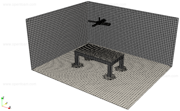
Here you can see the rotating and non-rotating regions of the mesh:

Now we move from the folder mesh to the folder case.
fixedFluxPressurefixedFluxPressurefixedFluxPressurefixedFluxPressureturbulentIntensityKineticEnergyInlet with 5% turbulence intensitykqRWallFunctionkqRWallFunctionkqRWallFunctionturbulentMixingLengthFrequencyInlet with 1.2m mixing lengthomegaWallFunctionomegaWallFunctionomegaWallFunctionnutkWallFunctionnutkWallFunctionnutkWallFunctioncellZone rotatingZone; - This was defined in snappyHexMeshDict to define the rotating cells.solidBodyMotionFunction rotatingMotion; - rotating mesh movementorigin (-3 2 2.6); - origin of the axis of rotation of cells (can be anywhere on the rotation axis of the fan)axis (0 0 1); - direction of the rotation axis (here: z-direction)omega 10; - angular velocity of rotation in rad/s= (corresponds to ~95.5 rpm)omega 20;The simulation employs the pimpleFoam application, in parallel.
decomposePar
With this command you divide your mesh and your fields onto multiple processors.
mpirun -np 4 pimpleFoam -parallel > log.pimpleFoam &
With this command you start your simulation on four cores. If you want to use a different number of cores you have to change the number (here: 4) to you choice. Also don't forget to change the settings in system/decomposeParDict!
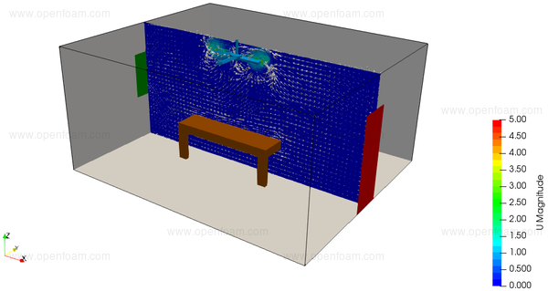
Here you see the flow after t = 0.64 s.
Velocity magnitude and vectors on a y-normal plane:
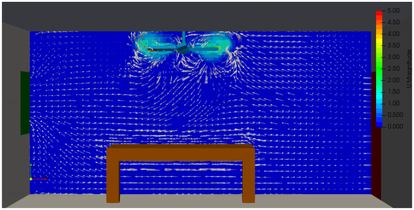
Close-up of velocity magnitude and vectors on a y-normal plane:
| Contributors to this page | Jozsef Nagy |
| Would you like to suggest an improvement to this page? | Create an issue |
Copyright © 2019 OpenCFD Ltd. and Contributors
Licensed under the Creative Commons License BY-NC-ND 
 1.8.17