The test case comprises a 2-D section comprising extruded triangle cells. An initial field is assigned the mesh cell centre values such that the computed gradient should take the value of 1 in each co-ordinate direction. By changing the choice of gradient scheme we can observe how each performs.
Gradient schemes under test:
Interpolation schemes under test:
Only the left and right domain boundaries are set to physical patch types; the remainder are set to the empty constraint to enforce the 2-D system.
The mesh comprises extruded triangle cells with low non-orthogonality with average and maximum values of 7 and 26 deg, respectively.
grad(Cc) <scheme>
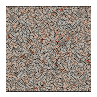
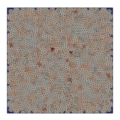
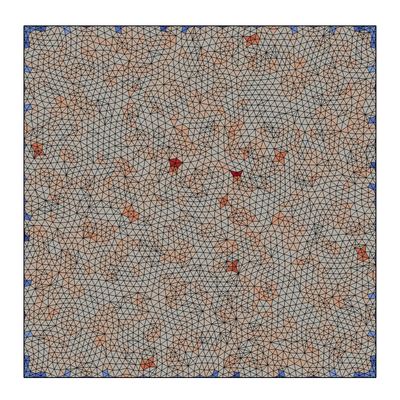
The following images show the percentage error of the magnitude of the gradient of the cell centres, defined as:
\[ \textrm{error} = 100 \frac{\left|\grad(C_c)\right| - 2^{0.5}}{2^{0.5}} \]
The range is set to +/- 10% for all images.
Gauss linear | 
Gauss point linear | 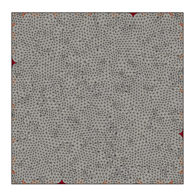
Least squares |

Gauss linear | 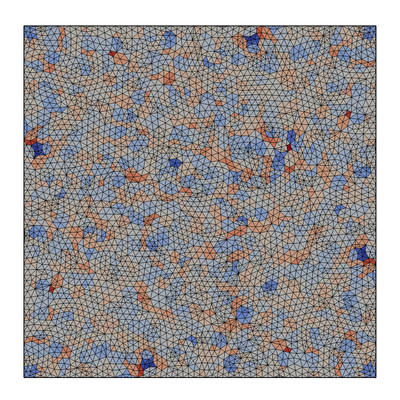
Gauss point linear | 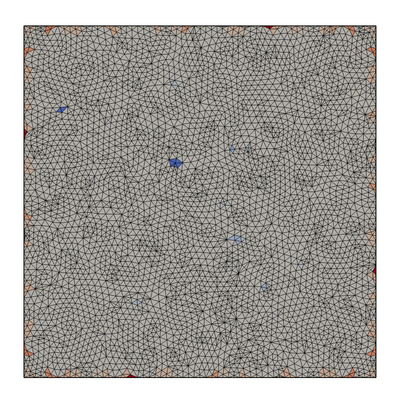
Least squares |
Gauss linear | 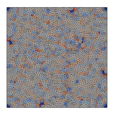
Gauss point linear | 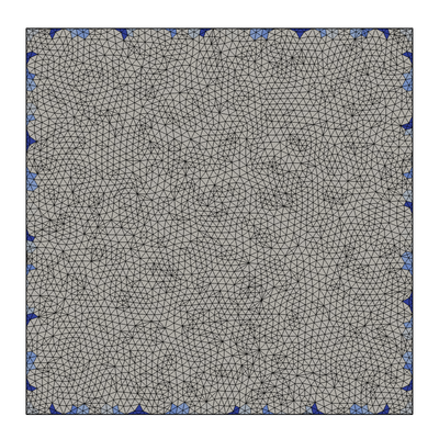
Least squares |

Gauss linear | 
Gauss point linear | 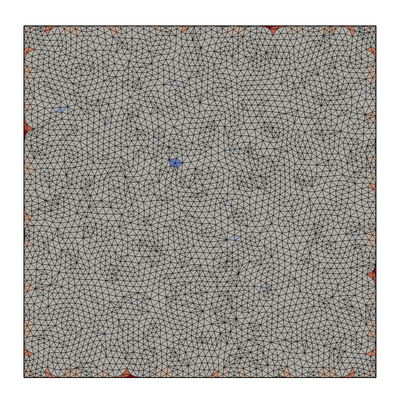
Least squares |
Gauss linear | 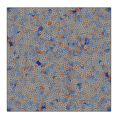
Gauss point linear | 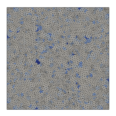
Least squares |
| Would you like to suggest an improvement to this page? | Create an issue |
Copyright © 2016 OpenCFD Ltd.
Licensed under the Creative Commons License BY-NC-ND 
 1.8.17